3: K-Nearest Neighbors (KNN)

3.1: K nearest neighbors

Assume we are given a dataset where \(X\) is a matrix of features from an observation and \(Y\) is a class label. We will use this notation throughout this article. \(k\)-nearest neighbors then, is a method of classification that estimates the conditional distribution of \(Y\) given \(X\) and classifies an observation to the class with the highest probability. Given a positive integer \(k\), \(k\)-nearest neighbors looks at the \(k\) observations closest to a test observation \(x_0\) and estimates the conditional probability that it belongs to class \(j\) using the formula

\[Pr(Y=j|X=x_0)=\frac{1}{k}\sum_{i\in \mathcal{N}_0}I(y_i=j)\]

where \(\mathcal{N}_0\) is the set of \(k\)-nearest observations and \(I(y_i=j)\) is an indicator variable that evaluates to 1 if a given observation \((x_i,y_i)\) in \(\mathcal{N}_0\) is a member of class \(j\), and 0 if otherwise. After estimating these probabilities, \(k\)-nearest neighbors assigns the observation \(x_0\) to the class which the previous probability is the greatest. The following plot can be used to illustrate how the algorithm works:

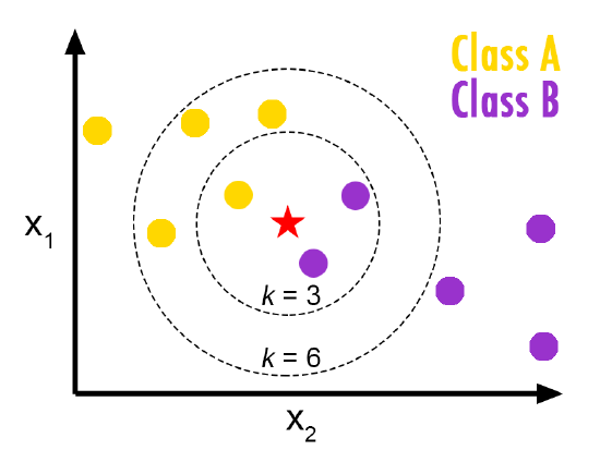
• If we choose \(K = 3\), then we have 2 observations in Class B and one observation in Class A. So, we classify the red star to Class B.
• If we choose \(K = 6\), then we have 2 observations in Class B but four observations in Class A. So, we classify the red star to Class A.

3.2: The Calculation of Distance

Since in k-NN algorithm, we need k nearest points, thus, the first step is calculating the distance between the input data point and other points in our training data. Suppose \(x\) is a point with coordinates \((x_1,x_2,...,x_p)\) and \(y\) is a point with coordinates \((y_1,y_2,...,y_p)\), then the distance between these two points is: \[d(x,y) = \sqrt{\sum_{i=1}^{p}(x_i - y_i)^2}\]

3.3: The Effect of K

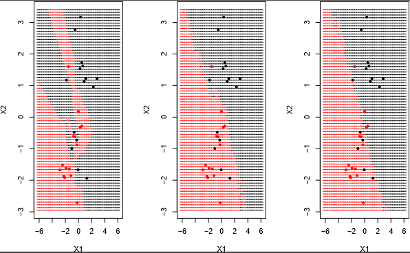
As most statistical learning model does, if \(K\) is small, then, we use a smaller region of data to learn. This may cause over-fitting.This may cause under-fitting. And if \(K\) is large, then we use a larger region of data to learn. The following plot shows the effects of \(K\). as \(K\) gets larger, the decision boundary appears linear.