
11.5: Biometrics Lab #5
- Page ID
- 2943

\( \newcommand{\vecs}[1]{\overset { \scriptstyle \rightharpoonup} {\mathbf{#1}} } \)
\( \newcommand{\vecd}[1]{\overset{-\!-\!\rightharpoonup}{\vphantom{a}\smash {#1}}} \)
\( \newcommand{\dsum}{\displaystyle\sum\limits} \)
\( \newcommand{\dint}{\displaystyle\int\limits} \)
\( \newcommand{\dlim}{\displaystyle\lim\limits} \)
\( \newcommand{\id}{\mathrm{id}}\) \( \newcommand{\Span}{\mathrm{span}}\)
( \newcommand{\kernel}{\mathrm{null}\,}\) \( \newcommand{\range}{\mathrm{range}\,}\)
\( \newcommand{\RealPart}{\mathrm{Re}}\) \( \newcommand{\ImaginaryPart}{\mathrm{Im}}\)
\( \newcommand{\Argument}{\mathrm{Arg}}\) \( \newcommand{\norm}[1]{\| #1 \|}\)
\( \newcommand{\inner}[2]{\langle #1, #2 \rangle}\)
\( \newcommand{\Span}{\mathrm{span}}\)
\( \newcommand{\id}{\mathrm{id}}\)
\( \newcommand{\Span}{\mathrm{span}}\)
\( \newcommand{\kernel}{\mathrm{null}\,}\)
\( \newcommand{\range}{\mathrm{range}\,}\)
\( \newcommand{\RealPart}{\mathrm{Re}}\)
\( \newcommand{\ImaginaryPart}{\mathrm{Im}}\)
\( \newcommand{\Argument}{\mathrm{Arg}}\)
\( \newcommand{\norm}[1]{\| #1 \|}\)
\( \newcommand{\inner}[2]{\langle #1, #2 \rangle}\)
\( \newcommand{\Span}{\mathrm{span}}\) \( \newcommand{\AA}{\unicode[.8,0]{x212B}}\)
\( \newcommand{\vectorA}[1]{\vec{#1}} % arrow\)
\( \newcommand{\vectorAt}[1]{\vec{\text{#1}}} % arrow\)
\( \newcommand{\vectorB}[1]{\overset { \scriptstyle \rightharpoonup} {\mathbf{#1}} } \)
\( \newcommand{\vectorC}[1]{\textbf{#1}} \)
\( \newcommand{\vectorD}[1]{\overrightarrow{#1}} \)
\( \newcommand{\vectorDt}[1]{\overrightarrow{\text{#1}}} \)
\( \newcommand{\vectE}[1]{\overset{-\!-\!\rightharpoonup}{\vphantom{a}\smash{\mathbf {#1}}}} \)
\( \newcommand{\vecs}[1]{\overset { \scriptstyle \rightharpoonup} {\mathbf{#1}} } \)
\(\newcommand{\longvect}{\overrightarrow}\)
\( \newcommand{\vecd}[1]{\overset{-\!-\!\rightharpoonup}{\vphantom{a}\smash {#1}}} \)
\(\newcommand{\avec}{\mathbf a}\) \(\newcommand{\bvec}{\mathbf b}\) \(\newcommand{\cvec}{\mathbf c}\) \(\newcommand{\dvec}{\mathbf d}\) \(\newcommand{\dtil}{\widetilde{\mathbf d}}\) \(\newcommand{\evec}{\mathbf e}\) \(\newcommand{\fvec}{\mathbf f}\) \(\newcommand{\nvec}{\mathbf n}\) \(\newcommand{\pvec}{\mathbf p}\) \(\newcommand{\qvec}{\mathbf q}\) \(\newcommand{\svec}{\mathbf s}\) \(\newcommand{\tvec}{\mathbf t}\) \(\newcommand{\uvec}{\mathbf u}\) \(\newcommand{\vvec}{\mathbf v}\) \(\newcommand{\wvec}{\mathbf w}\) \(\newcommand{\xvec}{\mathbf x}\) \(\newcommand{\yvec}{\mathbf y}\) \(\newcommand{\zvec}{\mathbf z}\) \(\newcommand{\rvec}{\mathbf r}\) \(\newcommand{\mvec}{\mathbf m}\) \(\newcommand{\zerovec}{\mathbf 0}\) \(\newcommand{\onevec}{\mathbf 1}\) \(\newcommand{\real}{\mathbb R}\) \(\newcommand{\twovec}[2]{\left[\begin{array}{r}#1 \\ #2 \end{array}\right]}\) \(\newcommand{\ctwovec}[2]{\left[\begin{array}{c}#1 \\ #2 \end{array}\right]}\) \(\newcommand{\threevec}[3]{\left[\begin{array}{r}#1 \\ #2 \\ #3 \end{array}\right]}\) \(\newcommand{\cthreevec}[3]{\left[\begin{array}{c}#1 \\ #2 \\ #3 \end{array}\right]}\) \(\newcommand{\fourvec}[4]{\left[\begin{array}{r}#1 \\ #2 \\ #3 \\ #4 \end{array}\right]}\) \(\newcommand{\cfourvec}[4]{\left[\begin{array}{c}#1 \\ #2 \\ #3 \\ #4 \end{array}\right]}\) \(\newcommand{\fivevec}[5]{\left[\begin{array}{r}#1 \\ #2 \\ #3 \\ #4 \\ #5 \\ \end{array}\right]}\) \(\newcommand{\cfivevec}[5]{\left[\begin{array}{c}#1 \\ #2 \\ #3 \\ #4 \\ #5 \\ \end{array}\right]}\) \(\newcommand{\mattwo}[4]{\left[\begin{array}{rr}#1 \amp #2 \\ #3 \amp #4 \\ \end{array}\right]}\) \(\newcommand{\laspan}[1]{\text{Span}\{#1\}}\) \(\newcommand{\bcal}{\cal B}\) \(\newcommand{\ccal}{\cal C}\) \(\newcommand{\scal}{\cal S}\) \(\newcommand{\wcal}{\cal W}\) \(\newcommand{\ecal}{\cal E}\) \(\newcommand{\coords}[2]{\left\{#1\right\}_{#2}}\) \(\newcommand{\gray}[1]{\color{gray}{#1}}\) \(\newcommand{\lgray}[1]{\color{lightgray}{#1}}\) \(\newcommand{\rank}{\operatorname{rank}}\) \(\newcommand{\row}{\text{Row}}\) \(\newcommand{\col}{\text{Col}}\) \(\renewcommand{\row}{\text{Row}}\) \(\newcommand{\nul}{\text{Nul}}\) \(\newcommand{\var}{\text{Var}}\) \(\newcommand{\corr}{\text{corr}}\) \(\newcommand{\len}[1]{\left|#1\right|}\) \(\newcommand{\bbar}{\overline{\bvec}}\) \(\newcommand{\bhat}{\widehat{\bvec}}\) \(\newcommand{\bperp}{\bvec^\perp}\) \(\newcommand{\xhat}{\widehat{\xvec}}\) \(\newcommand{\vhat}{\widehat{\vvec}}\) \(\newcommand{\uhat}{\widehat{\uvec}}\) \(\newcommand{\what}{\widehat{\wvec}}\) \(\newcommand{\Sighat}{\widehat{\Sigma}}\) \(\newcommand{\lt}{<}\) \(\newcommand{\gt}{>}\) \(\newcommand{\amp}{&}\) \(\definecolor{fillinmathshade}{gray}{0.9}\)Name: ______________________________________________________
You are working on an alternative energy source and biomass is a key component. You want to predict above-ground biomass for this region, and you believe that biomass is related to substrate (subsoil) variables of salinity, water acidity, potassium, sodium, and zinc. Your crew collects information on biomass and these five variables for 45 plots.
Experiment 1
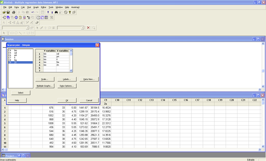
Before you create this regression model, you must examine the relationships between each of the five predictor variables and biomass (the response variable). Create five scatterplots using biomass as the response variable (y) and each of the predictor variables (x). Compute the linear correlation coefficient for each pair. Describe the relationships.
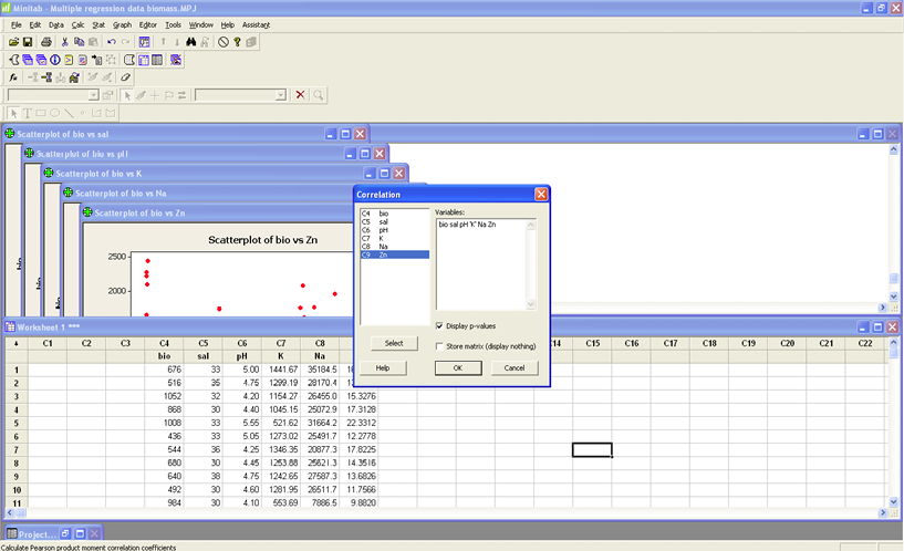
GRAPH>Scatterplot>Simple>OK. The response variable (y-variable) is Bio and the five predictor variables are the x-variables. Look at the scatterplots and describe each relationship below. Next compute the correlation coefficient for each pair and write the r-value below. STAT>Basic Statistics>Correlation. You can easily do all correlations at once by creating a correlation matrix. Put all predictor variables in the Variables box together.
Correlation (r) Description
Bio v. sal ______________________________________________________
Bio v.pH ______________________________________________________
Bio v. K _______________________________________________________
Bio v. Na ______________________________________________________
Bio v. Zn ______________________________________________________
Circle the above pair that has the strongest linear relationship.
Experiment 2
You are now going to create four regression models using the predictor variables. You will compare the adjusted R2, regression standard error, p-values for each coefficient, and the residuals for each model. Using this information, you will select the best model and state your reasons for this choice.
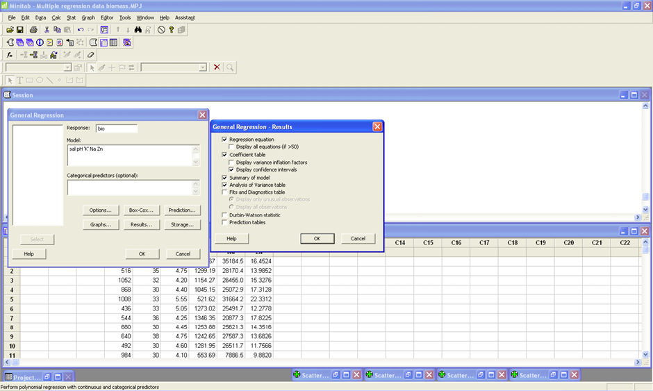
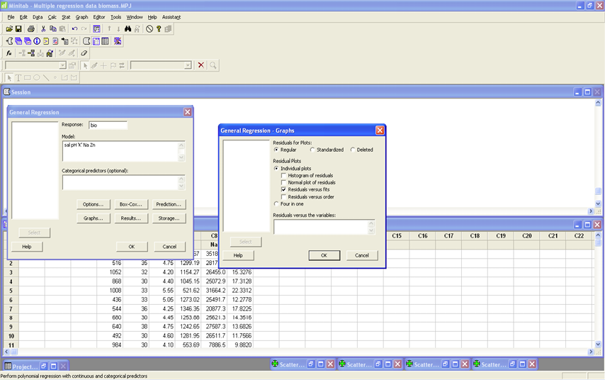
Begin with the full model using all five predictor variables. STAT>Regression>General Regression. Put Bio in the Response box and all five predictor variables in the Model box (see image). Click Results and make sure that the Regression equation, coefficient table, Display confidence intervals, Summary of Model, and Analysis of Variance Table are checked (see image). Click OK. Click Graphs and make sure that under Residual Plots that Individual plots and Residual versus Fits are selected (see image). Click OK.
MODEL 1
Write the regression model _______________________________________________
Write the adj. R2 ________________________________________________________
Write the regression standard error _________________________________________
Examine the residual plot. Are there any problems? ____________________________
Write the variables which are NOT significant ________________________________
MODEL 2
Now remove the LEAST significant variable (highest p-value) and repeat the steps using only the remaining variables.
Write the regression model _______________________________________________
Write the adj. R2 ________________________________________________________
Write the regression standard error _________________________________________
Examine the residual plot. Are there any problems? ____________________________
Write the variables which are NOT significant ________________________________
MODEL 3
Now remove the LEAST significant variable (highest p-value) and repeat the steps using only the remaining variables.
Write the regression model _______________________________________________
Write the adj. R2 ________________________________________________________
Write the regression standard error _________________________________________
Examine the residual plot. Are there any problems? ____________________________
Write the variables which are NOT significant ________________________________
MODEL 4
Now remove the LEAST significant variable (highest p-value) and repeat the steps using only the remaining variables.
Write the regression model _______________________________________________
Write the adj. R2 ________________________________________________________
Write the regression standard error _________________________________________
Examine the residual plot. Are there any problems? ____________________________
Write the variables which are NOT significant ________________________________
Experiment 3
Select the best model and state your reasons for selecting this model.
\[ \begin{array}{cccccc}
\text { biomass } & \text { sal } & \mathrm{pH} & \mathrm{K} & \mathrm{Na} & \mathrm{Zn} \\
676 & 33 & 5 & 1441.67 & 35184.5 & 16.4524 \\
516 & 35 & 4.75 & 1299.19 & 28170.4 & 13.9852 \\
1052 & 32 & 4.2 & 1154.27 & 26455 & 15.3276 \\
868 & 30 & 4.4 & 1045.15 & 25072.9 & 17.3128 \\
1008 & 33 & 5.55 & 521.62 & 31664.2 & 22.3312 \\
436 & 33 & 5.05 & 1273.02 & 25491.7 & 12.2778 \\
544 & 36 & 4.25 & 1346.35 & 20877.3 & 17.8225 \\
680 & 30 & 4.45 & 1253.88 & 25621.3 & 14.3516 \\
640 & 38 & 4.75 & 1242.65 & 27587.3 & 13.6826 \\
492 & 30 & 4.6 & 1281.95 & 26511.7 & 11.7566 \\
984 & 30 & 4.1 & 553.69 & 7886.5 & 9.882 \\
1400 & 37 & 3.45 & 494.74 & 14596 & 16.6752 \\
1276 & 33 & 3.45 & 525.97 & 9826.8 & 12.373 \\
1736 & 36 & 4.1 & 571.14 & 11978.4 & 9.4058 \\
1004 & 30 & 3.5 & 408.64 & 10368.6 & 14.9302 \\
396 & 30 & 3.25 & 646.65 & 17307.4 & 31.2865 \\
352 & 27 & 3.35 & 514.03 & 12822 & 30.1652 \\
328 & 29 & 3.2 & 350.73 & 8582.6 & 28.5901 \\
392 & 34 & 3.35 & 496.29 & 12369.5 & 19.8795 \\
236 & 36 & 3.3 & 580.92 & 14731.9 & 18.5056 \\
392 & 30 & 3.25 & 535.82 & 15060.6 & 22.1344 \\
268 & 28 & 3.25 & 490.34 & 11056.3 & 28.6101 \\
252 & 31 & 3.2 & 552.39 & 8118.9 & 23.1908 \\
236 & 31 & 3.2 & 661.32 & 13009.5 & 24.6917 \\
340 & 35 & 3.35 & 672.15 & 15003.7 & 22.6758 \\
2436 & 29 & 7.1 & 528.65 & 10225 & 0.3729 \\
2216 & 35 & 7.35 & 563.13 & 8024.2 & 0.2703 \\
2096 & 35 & 7.45 & 497.96 & 10393 & 0.3205 \\
1660 & 30 & 7.45 & 458.38 & 8711.6 & 0.2648 \\
2272 & 30 & 7.4 & 498.25 & 10239.6 & 0.2105 \\
824 & 26 & 4.85 & 936.26 & 20436 & 18.9875 \\
1196 & 29 & 4.6 & 894.79 & 12519.9 & 20.9687 \\
1960 & 25 & 5.2 & 941.36 & 18979 & 23.9841 \\
2080 & 26 & 4.75 & 1038.79 & 22986.1 & 19.9727 \\
1764 & 26 & 5.2 & 898.05 & 11704.5 & 21.3864 \\
412 & 25 & 4.55 & 989.87 & 17721 & 23.7063 \\
416 & 26 & 3.95 & 951.28 & 16485.2 & 30.5589 \\
504 & 26 & 3.7 & 939.83 & 17101.3 & 26.8415 \\
492 & 27 & 3.75 & 925.42 & 17849 & 27.7292 \\
636 & 27 & 4.15 & 954.11 & 16949.6 & 21.5699 \\
1756 & 24 & 5.6 & 720.72 & 11344.6 & 19.6531 \\
1232 & 27 & 5.35 & 782.09 & 14752.4 & 20.3295 \\
1400 & 26 & 5.5 & 773.3 & 13649.8 & 19.588 \\
1620 & 28 & 5.5 & 829.26 & 14533 & 20.1328 \\
1560 & 28 & 5.4 & 856.96 & 16892.2 & 19.242
\end{array} \nonumber \]