18.6: Compare two linear models

Rcmdr (R) provides a very useful tool to compare models. Now, you can compare any two models, but this would be a poor strategy. Use this tool to perform in effect a stepwise test by hand. As one of the models, select for example the saturated model, then for the second model, select one in which you drop one model factor. In the example below, I dropped the two-way interaction from the saturated model (a logistic regression model, actually):

The model was \[Type.II diabetes ~ Treatment + Samples + Gender + BMI + Age + Gender:Treatment \nonumber\]

where Type.II diabetes is a binomial (Yes,No) dependent variable and Treatment and Gender were categorical factors. The ANOVA table is shown below.

Anova(GLM.1, type="II", test="LR")
Analysis of Deviance Table (Type II tests)
Response: Type.II
                LR Chisq  Df Pr(>Chisq)
Treatment          0.266  7    0.9999
Samples           38.880  1    4.508e-10 ***
Gender             0.671  1    0.4127
BMI                2.259  1    0.1329
Age                2.064  1    0.1508
Treatment:Gender   1.803  1    0.1794

From this output we see that there are a number of terms that are not significant \((P < 0.05)\), but with one exception (Treatment) they seem to contribute to the total variation (\(P\) values are between 0.13 and 0.4). So, we conclude that the saturated model is not the best fit model, and proceed to evaluate alternative models in search of the best one.

As a matter of practice I first drop the interaction term. Here’s the ANOVA table for the second model, now without the interaction:

Anova(GLM.1, type="II", test="LR")
Analysis of Deviance Table (Type II tests)
Response: Type.II
              LR Chisq Df Pr(>Chisq)
Treatment        0.266  7    0.9999
Samples         37.086  1    1.13e-09 ***
Gender           0.671  1    0.4127
BMI              2.017  1    0.1556
Age              1.794  1    0.1804

Both models look about the same. Which one is best? We now wish to know if dropping the interaction harms the model in any way. We will use the AIC (Akaike Information Criterion) to evaluate the models. AIC provides a way to assess which among a set of nested models is better. The preferred model is the one with the lowest AIC value.

To access the AIC calculation, just enter the script AIC(model name), where model name refers to one of the models you wish to evaluate (e.g., GLM.1), then submit the code

AIC(GLM.1)
50.65518

AIC(GLM.2)
50.45793

Thus, we prefer the second model (GLM.2) because the AIC is lower.

AIC does not provide a statistical test of model fit. To access the model comparison tool, simply select

Models → Hypothesis tests → Compare two models…

and the following screen will appear.

Figure \(\PageIndex{1}\): Compare Models menu in R Commander.

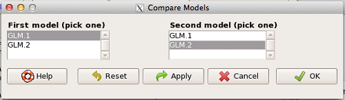
Select the two models to compare (in this case, GLM1 and GLM2), then press OK button. R output:

anova(GLM.1, GLM.2, test="Chisq")
Analysis of Deviance Table
Model 1: Type.II ~ Treatment + Samples + Gender + BMI + Age + Gender:Treatment
Model 2: Type.II ~ Treatment + Samples + Gender + BMI + Age
    Resid. Df  Resid. Dev  Df  Deviance P(>|Chi|)
1          49      24.655
2          50      26.458  -1   -1.8027   0.1794

We see that \(P > 0.05 (= 0.1794)\), which means the fit of the model is fine if we lose the one term.

Deviance

Those of you working with logistic regressions will see this new term, “deviance.” Deviance is a statistical term relevant to model fitting. Think of it like a chi-square test statistic. The idea is that you compare your fitted model against the data in which the only thing estimate is the intercept. Do the additional components of the model add significantly to the prediction of the original data? If they do, dropping the term will have a significant effect on the model fit and the P-value would be less than 0.05. In this example, we see that dropping the interaction term had little effect on the deviance score and in agreement, the P value is larger than 0.05. It means we can drop the term and the new model lacking the term is in some sense better: fewer predictors, a simpler model.

Questions

[pending]