12.6: ANOVA post-hoc tests

ANOVA post-hoc tests

Tests of the null hypothesis in a one-way ANOVA yields one answer: either you reject the null, or you do not reject the null hypothesis.

But while there was only one factor (population, drug treatment, etc) in a one-way ANOVA, there are usually many treatments (e.g., multiple levels, four different populations, 3 doses of a drug plus a placebo). ANOVA plus post-hoc tests solves the multiple comparison problem we discussed: you still get your tests of all group differences, but with adjustments to the procedures so that these tests are conducted without suffering the increase in type I error = the multiple comparison problem. If the null hypothesis is rejected, you may then proceed to post-hoc tests among the groups to identify differences.

Consider the following example of four populations scored for some outcome, sim.ch12 (scroll down the page, or click here to get the R code).

Bring the data frame, sim.ch12, into current memory in Rcmdr by selecting the data set. Next, run the one-way ANOVA.

Rcmdr: Statistics → Means → One-way ANOVA…

which brings up the following menu (Fig. \(\PageIndex{1}\))

Figure \(\PageIndex{1}\): One-way ANOVA menu in R Commander.

Note:

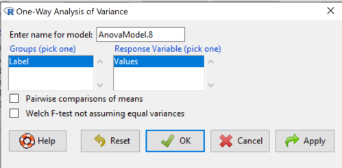
If you look carefully in Figure \(\PageIndex{1}\), you can see model name was AnovaModel.8. There’s nothing significant about that name, it just means this was the 8^th model I had run up to that point. As a reminder, Rcmdr will provide names for models for you; it is better practice to provide model names yourself.

Notice that Rcmdr menu correctly identifies the Factor variable, which contains text labels for each group, and the Response variable, which contains the numerical observations.

Note:

If your factor is numeric, you’ll first have to tell R that the variable is a factor and hence nominal. this can be accomplished within Rcmdr via the Data Manage variables… options, or simply submit the command

newName <- as.factor(oldVariable)

If your data set contains more variables, then you would need to sort through these and select the correct model (Fig. \(\PageIndex{1}\)).

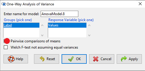
To get the default Tukey post-hoc tests simply check the Pairwise comparisons box and then click OK.

For a test of the null that four groups have the same mean, a publishable ANOVA table would look like…

Table \(\PageIndex{1}\). The ANOVA table.

	Df	Mean Square	F	P†
Label	3	389627	76.44	< 0.0001
Error	36	61167

† Dr. D edited the R output for p-value. R doesn’t report P as less than some value.

Note:

The ANOVA table is something you put together from the output of R (or other statistical programs).

Here’s the R output for ANOVA:

AnovaModel.8 <- aov(Values ~ Label, data = sim.Ch12)
summary(AnovaModel.8)
          Df  Sum Sq Mean Sq  F value     Pr(>F) 
Label      3  389627  129876    76.44   1.11e-15 ***
Residuals 36   61167    1699 
---
Signif. codes: 0 '***' 0.001 '**' 0.01 '*' 0.05 '.' 0.1 ' ' 1

with(sim.Ch12, numSummary(Values, groups = Label, statistics = c("mean", "sd")))
      mean       sd data:n
Pop1 150.3 35.66838 10
Pop2  99.0 43.25634 10
Pop3 130.9 42.36469 10
Pop4 350.7 43.10723 10

End of R output.

Recall that all we can say is that a difference has been found and we reject the null hypothesis. However, we do not know if group 1 = group 2, but both are different from group 3, or some other combination. So we need additional tools. We can conduct post-hoc tests (also called multiple comparisons tests).

Once a difference has been detected (\(F\) test statistic > \(F\) critical value, therefore \(P < 0.05\)), then posteriori tests, also called unplanned comparisons, can be used to tell which means differ.

There are also cases for which some comparisons were planned ahead of time and these are called a priori or planned comparisons; even though you conduct the tests after the ANOVA, you were always interested in particular comparisons. This is an important distinction: planned comparisons are more powerful, more aligned with what we understand to be the scientific method.

Let’s take a look at these procedures. Collectively, they are often referred to as post-hoc tests (Ruxton and Beauchamp 2008). There are many different flavors of these tests, and R offers several, but I will hold you responsible only for three such comparisons: Tukey’s, Dunnett’s, and Bonferroni (Dunn). These named tests are among the common ones, but you should be aware that the problem of multiple comparisons and inflated error rates has received quite a lot of recent attention because the size of data sets has increased in many fields, e.g., genome wide-association studies in genetics or data mining in economics or business analytics. A related topic then is the issue of “false positives.” New approaches include Holm-Bonferroni. There are others — it is a regular “cottage industry” in applied statistics to a problem that, while recognized, has not achieved a universal agreed solution. Best we can do is be aware and deal with it and know that the problem is one mostly of big data (e.g., microarray and other high-through put approaches).

Important R Note: In order to do most of the post-hoc tests you will need to install the multcomp package; after installing the package, load the library(multcomp). Just using the default option from the one-way ANOVA command yields the Tukey’s HSD test.

Performing multiple comparisons and the one-way ANOVA

a. Tukey’s: “honestly (wholly) significant difference test”

Tests \(H_{O}: \bar{X}_{B} = \bar{X}_{A}\) versus \(H_{A}: \bar{X}_{B} \neq \bar{X}_{A}\) where \(A\) and \(B\) can be any pairwise combination of two means you wish to compare. There are \(\frac{k(k-1)}{2}\) comparisons.

\[q = \frac{\bar{X}_{B} - \bar{X}_{A}}{SE} \nonumber\]

where \[SE = \sqrt{\frac{MS_{error}}{n}} \nonumber\]

and \(n\) is the harmonic mean of the sample sizes of the two groups being compared. If the sample sizes are equal, then the simple arithmetic mean is the same as the harmonic mean.

Note:

\(q\) is like \(t\) for when we are testing means from two samples.

• The significance level is the probability of encountering at least one Type I error (probability of rejecting \(H_{O}\) when it is true). This is called the experiment-wise (family-wise) error rate whereas before we talked about the comparison-wise (individual) error rate.

Two options to get the post-hoc test Tukey — use a package called mcp or in Rcmdr, Tukey is the default option in the one-way ANOVA command.

Rcmdr: Statistics → Means → One-way ANOVA
Check “Pairwise comparisons of means” to get the Tukey’a HSD test (Fig. \(\PageIndex{2}\))

Figure \(\PageIndex{2}\): Select Tukey post-hoc tests with the one-way ANOVA.

R output follows. There’s a lot, but much of it is repeat information. Take your time, here we go.

.Pairs <- glht(AnovaModel.4, linfct = mcp(Label = "Tukey"))
summary(.Pairs) # pairwise tests
     Simultaneous Tests for General Linear Hypotheses
Multiple Comparisons of Means: Tukey Contrasts
 Fit: aov(formula = Values ~ Label, data = sim.Ch12) 

 Linear Hypotheses: 
                  Estimate Std. Error t value Pr(>|t|)     
 Pop2 - Pop1 == 0   -51.30      18.43  -2.783   0.0405 *   
 Pop3 - Pop1 == 0   -19.40      18.43  -1.052   0.7201     
 Pop4 - Pop1 == 0   200.40      18.43  10.871   <0.001 *** 
 Pop3 - Pop2 == 0    31.90      18.43   1.730   0.3233     
 Pop4 - Pop2 == 0   251.70      18.43  13.654   <0.001 *** 
 Pop4 - Pop3 == 0   219.80      18.43  11.924   <0.001 *** 
 --- 
 Signif. codes:  0 '***' 0.001 '**' 0.01 '*' 0.05 '.' 0.1 ' ' 1 
 (Adjusted p values reported -- single-step method) 

 confint(.Pairs) # confidence intervals 
      Simultaneous Confidence Intervals 

 Multiple Comparisons of Means: Tukey Contrasts 

 Fit: aov(formula = Values ~ Label, data = sim.Ch12) 

 Quantile = 2.6927 
 95% family-wise confidence level 
   
 Linear Hypotheses: 
                  Estimate  lwr       upr       
 Pop2 - Pop1 == 0  -51.3000 -100.9382   -1.6618 
 Pop3 - Pop1 == 0  -19.4000  -69.0382   30.2382 
 Pop4 - Pop1 == 0  200.4000  150.7618  250.0382 
 Pop3 - Pop2 == 0   31.9000  -17.7382   81.5382 
 Pop4 - Pop2 == 0  251.7000  202.0618  301.3382 
 Pop4 - Pop3 == 0  219.8000  170.1618  269.4382 

Figure \(\PageIndex{3}\): Plot of confidence intervals of Tukey HSD.

R Commander includes a default 95% CI plot (Fig. \(\PageIndex{3}\)). From this graph, you can quickly identify the pairwise comparisons for which 0 (zero, dotted vertical line) is included in the interval, i.e., there is no difference between the means (e.g., Pop1 is different from Pop4, but Pop1 is not different from Pop3).

b. Dunnett’s Test for comparisons against a control group

• There are situations where we might want to compare our experimental Populations to one control Population or group.
• This is common in medical research where there is a placebo (control pill with no drug) or sham operations (operations where every thing but the critical operation is done).
• This is also a common research design in ecological or agricultural research where some animal or plant populations are exposed to an environmental factor (e.g. fertilizer, pesticide, pollutant, competitors, herbivores) and other animal or plant populations are not exposed to these environmental factor.
• The difference in the statistical procedure for analyzing this type of research design is that the experimental groups may only be compared to the control group.
• This results in fewer comparisons.
• The formula is the same as for the Tukey’s Multiple Comparison test, except for the calculation of the \(SE\).

Standard Error is changed by multiplying the \(MS_{Error}\) by 2.

And \(n\) is the harmonic mean of the sample sizes of the two groups being compared. \[q = \frac{\bar{X}_{control} - \bar{X}_{A}}{SE} \nonumber\]

where \[SE = \sqrt{\frac{2 / MS_{error}}{n}} \nonumber\]

R Commander doesn’t provide a simple way to get Dunnett, but we can get it simply enough if we are willing to write some script. Fortunately (OK, by design!), Rcmdr prints commands.

Look at the Output window from the one-way ANOVA with pairwise comparisons: it provides clues as to how we can modify the mcp command (mcp stands for multiple comparisons).

First, I had run the one-way ANOVA command and noted the model (AnovaModel.3). Second, I wrote the following script, modified from above.

Pairs <- glht(AnovaModel.1, linfct = mcp(Label = c("Pop2 - Pop1 = 0", "Pop3 - Pop1 = 0", "Pop4 - Pop1 = 0")))

where Label is my name for the Factor variable. Note that I specified the comparisons I wanted R to make. When I submit the script, nothing shows up in the Output window because the results are stored in my “Pairs.”

I then need to ask R to provide confidence intervals

confint(Pairs)

R output window

Pairs <- glht(AnovaModel.1, linfct = mcp(Label = c("Pop2 - Pop1 = 0", "Pop3 - Pop1 = 0", "Pop4 - Pop1 = 0"))) 
confint(Pairs) 

Simultaneous Confidence Intervals 

 Multiple Comparisons of Means: User-defined Contrasts 

 Fit: aov(formula = Values ~ Label, data = sim.Ch12) 

 Estimated Quantile = 2.4524 
 95% family-wise confidence level 

 Linear Hypotheses: 
  ...... lwr ....... upr 
 Pop2 - Pop1 == 0  .. -51.3000  . -96.5080  ... -6.0920 
 Pop3 - Pop1 == 0  .. -19.4000  . -64.6080  ... 25.8080 
 Pop4 - Pop1 == 0  .. 200.4000  . 155.1920  .. 245.6080

Look for intervals that include zero, therefore, the group does not differ from the Control group (Pop1). How many groups differed from the Control group?

Alternatively, I may write

Tryme <- glht(AnovaModel.1, linfct = mcp(Label = "Dunnett"))
confint(Tryme)

It’s the same (in fact, the default mcp test is the Dunnett).

Tryme <- glht(AnovaModel.1, linfct = mcp(Label = "Dunnett")) 
confint(Tryme) 

Simultaneous Confidence Intervals 

Multiple Comparisons of Means: Dunnett Contrasts 

Fit: aov(formula = Values ~ Label, data = sim.Ch12) 

Estimated Quantile = 2.4514 
95% family-wise confidence level 

Linear Hypotheses: 
Estimate lwr upr 
Pop2 - Pop1 == 0 -51.3000 -96.4895 -6.1105 
Pop3 - Pop1 == 0 -19.4000 -64.5895 25.7895 
Pop4 - Pop1 == 0 200.4000 155.2105 245.5895                                   

c. Bonferroni \(t\)

The Bonferroni t test is a popular tool for conducting multiple comparisons. The rationale for this particular test is that the \(MS_{error}\) is a good estimate of the pooled variances for all groups in the ANOVA.

\[Bonferroni = \frac{\bar{X}_{B} - \bar{X}_{A}}{\sqrt{MS_{error} \left(\frac{1}{n_{B}} + \frac{1}{n_{A}}\right)}} \nonumber\]

and \(DF = N - k\).

Note:

In order to achieve a Type I error rate of 5% for all tests, you must divide the 0.05 by the number of comparisons conducted.

Thus, for \(k = 4\) groups, \(\left(^{4}_{2}\right) = \frac{4!}{2! (4-2)!}\)

Here’s a more general version if you prefer to get all pairwise tests: \(\left(^{k}_{2}\right) = \frac{k!}{2! (k-2)!}\)

Use this information then to determine how many total comparisons will be made, then if necessary, use to adjust Type I error rate for one test (the exeriment-wise error rate).

For our example, the adjusted Type I error is \(0.05/6 = 0.00833\). Thus, for a difference between two means to be statistically significant, the P-value must be less than 0.00833.

For Bonferroni, we will use the following script.

1. Set up one-way ANOVA model (ours has been saved as AnovaModel.1),
2. Collect all pairwise comparisons with the mcp(~”Tukey”) stored in a vector (I called mine Whynot),
3. and finally, get the Bonferroni adjusted test of the comparisons with the summary command, but add the “test = adjusted(“bonferroni”).

It’s a bit much, but we end up with a very nice output to work with.

Whynot <- glht(AnovaModel.3, linfct = mcp(Label = "Tukey")) 
summary(Whynot, test = adjusted("bonferroni")) 

 Simultaneous Tests for General Linear Hypotheses

Multiple Comparisons of Means: Tukey Contrasts

Fit: aov(formula = Values ~ Label, data = sim.Ch12)

Linear Hypotheses:
Estimate Std. Error t value Pr(>|t|) 
Pop2 - Pop1 == 0 -51.30 18.43 -2.783 0.0512 . 
Pop3 - Pop1 == 0 -19.40 18.43 -1.052 1.0000 
Pop4 - Pop1 == 0 200.40 18.43 10.871 3.82e-12 ***
Pop3 - Pop2 == 0 31.90 18.43 1.730 0.5527 
Pop4 - Pop2 == 0 251.70 18.43 13.654 5.33e-15 ***
Pop4 - Pop3 == 0 219.80 18.43 11.924 2.77e-13 ***
  --- 
 Signif. codes: 0 '***' 0.001 '**' 0.01 '*' 0.05 '.' 0.1 ' ' 1 
 (Adjusted p values reported -- bonferroni method)        

---

Questions

1. Be able to define and contrast experiment-wise and family-wise error rates.
2. Read and interpret R output
   1. Refer back to the Tukey HSD output. Among the four populations, which pairwise groups were considered “statistically significant” following use of the Tukey HSD?
   2. Refer back to the Dunnett’s output. Among the four populations, which population was taken as the control group for comparison?
   3. Refer back to the Dunnett’s output. Which pairwise groups were considered “statistically significant” from the control group?
   4. Refer back to the Bonferroni output. Among the four populations, which pairwise groups were considered “statistically significant” following use of the Bonferroni correction?
   5. Compare and contrast interpretation of results for post-hoc comparisons among the four populations based on the three different post-hoc methods
3. Be able to distinguish when Tukey HSD and Dunnet’s post hoc tests are appropriate.
4. Some microarray researchers object to use of Bonferroni correction because it is too “conservative.” In the context of statistical testing, what errors are the researchers talking about when they say the correction is “conservative”?

---

Data set used in this page

sim.ch12 <- read.table(header=TRUE, sep=",",text="
Label, Value
Pop1, 105
Pop1, 132
Pop1, 156
Pop1, 198
Pop1, 120
Pop1, 196
Pop1, 175
Pop1, 180
Pop1, 136
Pop1, 105
Pop2, 100
Pop2, 65
Pop2, 60
Pop2, 125
Pop2, 80
Pop2, 140
Pop2, 50
Pop2, 180
Pop2, 60
Pop2, 130
Pop3, 130
Pop3, 95
Pop3, 100
Pop3, 124
Pop3, 120
Pop3, 180
Pop3, 80
Pop3, 210
Pop3, 100
Pop3, 170
Pop4, 310
Pop4, 302
Pop4, 406
Pop4, 325
Pop4, 298
Pop4, 412
Pop4, 385
Pop4, 329
Pop4, 375
Pop4, 365")
#check the dataframe
head(sim.ch12)