11.5: Power analysis in R

Introduction

In R, you can estimate the

1. Statistical power — how probable are you to correctly reject the null hypothesis?
2. Sample size — how many samples or observations must we get to have a reasonable chance to correctly reject a null hypothesis?
3. Effect size (minimum difference) — how different are the two samples?

Power analysis is recommended before conducting an experiment, but it is also valuable after an experiment.

Base R and pwr package

In Chapter 11.4 we presented functions from BSDA package. R (but not Rcmdr, but see the EZR plugin described below) provides all of the basic power analysis we would need for t-tests, one-way ANOVA, etc. as part of the base installation (Everitt and Hothorn 2007). However, the package pwr, provides a more comprehensive package for power analysis. Load and install the R package pwr.

For example, to determine the number of samples for an independent sample t-test (two-tailed), the function is pwr.t.test().

pwr.t.test(n = NULL, d = NULL, sig.level = 0.05, power = NULL, type = c("two.sample", "one.sample", "paired"), alternative = c("two.sided", "less","greater"))

Table \(\PageIndex{1}\). Parameters of the pwr.t.test()function.

n	Number of observations (per sample)
d	Effect size
sig.level	Significance level (Type I error probability)
power	Power of test (1 minus Type II error probability)
type	Type of t-test : one-, two-, or paired-samples
alternative	a character string specifying the alternative hypothesis, must be one of “two.sided” (default), “greater” or “less”

The basic question is, how many samples (observations) do I need for each group (k) at Type I error of 5% and type II error of 95%?

To run the test, you fill in all of the “NULL” except the one you wanted solved (i.e., leave n = NULL).

For an effect size of 0.2, Type I error (significance level) of 5%, and 95% power, how many observations per group do we need for our study?

pwr.t.test(n = NULL, d =0.2, sig.level = 0.05, power = 0.95, type = c("two.sample"), alternative = c("two.sided"))
Two-sample t test power calculation
n = 650.6974
d = 0.2
sig.level = 0.05 power = 0.95 alternative = two.sided

note: n is number “n” in each group

Wow!

The R pwr package is not as convenient as it could be (have to load and run R scripts): for intro level, try one of the many online sites. Here is a website which can help with power analysis based on a variety of situations. The programs are java-coded. http://www.stat.uiowa.edu/~rlenth/Power/index.html

Power analysis with the EZR Rcmdr plugin

The EZR plugin for R Commander provides some facilities to do power analysis (Kanda 2013). First, download and install the RcmdrPlugin.EZR package. The EZR plugin for Rcmdr, RcmdrPlugin.EZR, provides an interface to explore power analyses, along with many other statistical functions (Kanda 2013). After loading the plugin to Rcmdr, additional drop down options are added to the menu bar (Fig. \(\PageIndex{1}\)).

Figure \(\PageIndex{1}\): Screenshot of Rcmdr menu bar with (A) and without (B) the EZR plugin.

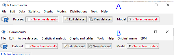
I’ll demonstrate use of the plugin, but I recommend that you use pwr.t.test() instead. Although EZR uses a drop-down menu system, it has many more functions than we need to solve this simple exercise. Thus, EZR is not any easier to apply for what we need here. That said, off we go.

Worked example

Consider a simple data set: wheel running performance in 24 hours for three strains of mice.

Table \(\PageIndex{2}\). Wheel running performance in 24 hours for three strains of mice.

Mouse strain	Average	Standard deviation	n
AKR	395	169.7	20
CBA	855	77.8	20
C57BL/10	1135	63.6	20

Consider two groups of mice, AKR vs CBA for wheel running performance. How many samples are needed to show a statistical difference for performances between the two groups?

Calculate the pooled standard deviation and calculate a difference between the means (the effect size) for which you wish to say is statistically different. For this example, 132.0 and 460, respectively. With EZR plugin installed and active in R Commander (Fig. \(\PageIndex{2}\)), select

Rcmdr: Statistical analysis → Calculate sample size → Calculate sample size for comparison between two means

Figure \(\PageIndex{2}\): Screenshot of Rcmdr EZR plugin menu.

Select “Calculate sample size for comparison between two means”, enter the effect size (Difference in means), standard deviation in each group (or a single value for pooled standard deviation), alpha error, power, and sample size ratio.

Figure \(\PageIndex{2}\): Screenshot of EZR Menu to obtain sample size for the AKR vs CBA data.

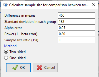
R output from EZR Calculate sample size for comparison between two means:

Assumptions
Difference in means 460
Standard deviation 132
Alpha 0.05
two-sided
Power 0.8
N2/N1 1

Required sample size Estimated
N1 2
N2 2

---

Questions

Recall the lizard body mass data set from Chapter 10.1

Geckos <- c(3.186, 2.427, 4.031, 1.995)
Anoles <- c(5.515, 5.659, 6.739, 3.184)

Enter the data into an R data.frame, carry out the independent sample t-test, then

1. Calculate power for the comparison between the two means
2. Calculate sample size needed to achieve 95% power.