
5.2: The Normal Distribution
- Page ID
- 7226

\( \newcommand{\vecs}[1]{\overset { \scriptstyle \rightharpoonup} {\mathbf{#1}} } \)
\( \newcommand{\vecd}[1]{\overset{-\!-\!\rightharpoonup}{\vphantom{a}\smash {#1}}} \)
\( \newcommand{\dsum}{\displaystyle\sum\limits} \)
\( \newcommand{\dint}{\displaystyle\int\limits} \)
\( \newcommand{\dlim}{\displaystyle\lim\limits} \)
\( \newcommand{\id}{\mathrm{id}}\) \( \newcommand{\Span}{\mathrm{span}}\)
( \newcommand{\kernel}{\mathrm{null}\,}\) \( \newcommand{\range}{\mathrm{range}\,}\)
\( \newcommand{\RealPart}{\mathrm{Re}}\) \( \newcommand{\ImaginaryPart}{\mathrm{Im}}\)
\( \newcommand{\Argument}{\mathrm{Arg}}\) \( \newcommand{\norm}[1]{\| #1 \|}\)
\( \newcommand{\inner}[2]{\langle #1, #2 \rangle}\)
\( \newcommand{\Span}{\mathrm{span}}\)
\( \newcommand{\id}{\mathrm{id}}\)
\( \newcommand{\Span}{\mathrm{span}}\)
\( \newcommand{\kernel}{\mathrm{null}\,}\)
\( \newcommand{\range}{\mathrm{range}\,}\)
\( \newcommand{\RealPart}{\mathrm{Re}}\)
\( \newcommand{\ImaginaryPart}{\mathrm{Im}}\)
\( \newcommand{\Argument}{\mathrm{Arg}}\)
\( \newcommand{\norm}[1]{\| #1 \|}\)
\( \newcommand{\inner}[2]{\langle #1, #2 \rangle}\)
\( \newcommand{\Span}{\mathrm{span}}\) \( \newcommand{\AA}{\unicode[.8,0]{x212B}}\)
\( \newcommand{\vectorA}[1]{\vec{#1}} % arrow\)
\( \newcommand{\vectorAt}[1]{\vec{\text{#1}}} % arrow\)
\( \newcommand{\vectorB}[1]{\overset { \scriptstyle \rightharpoonup} {\mathbf{#1}} } \)
\( \newcommand{\vectorC}[1]{\textbf{#1}} \)
\( \newcommand{\vectorD}[1]{\overrightarrow{#1}} \)
\( \newcommand{\vectorDt}[1]{\overrightarrow{\text{#1}}} \)
\( \newcommand{\vectE}[1]{\overset{-\!-\!\rightharpoonup}{\vphantom{a}\smash{\mathbf {#1}}}} \)
\( \newcommand{\vecs}[1]{\overset { \scriptstyle \rightharpoonup} {\mathbf{#1}} } \)
\(\newcommand{\longvect}{\overrightarrow}\)
\( \newcommand{\vecd}[1]{\overset{-\!-\!\rightharpoonup}{\vphantom{a}\smash {#1}}} \)
\(\newcommand{\avec}{\mathbf a}\) \(\newcommand{\bvec}{\mathbf b}\) \(\newcommand{\cvec}{\mathbf c}\) \(\newcommand{\dvec}{\mathbf d}\) \(\newcommand{\dtil}{\widetilde{\mathbf d}}\) \(\newcommand{\evec}{\mathbf e}\) \(\newcommand{\fvec}{\mathbf f}\) \(\newcommand{\nvec}{\mathbf n}\) \(\newcommand{\pvec}{\mathbf p}\) \(\newcommand{\qvec}{\mathbf q}\) \(\newcommand{\svec}{\mathbf s}\) \(\newcommand{\tvec}{\mathbf t}\) \(\newcommand{\uvec}{\mathbf u}\) \(\newcommand{\vvec}{\mathbf v}\) \(\newcommand{\wvec}{\mathbf w}\) \(\newcommand{\xvec}{\mathbf x}\) \(\newcommand{\yvec}{\mathbf y}\) \(\newcommand{\zvec}{\mathbf z}\) \(\newcommand{\rvec}{\mathbf r}\) \(\newcommand{\mvec}{\mathbf m}\) \(\newcommand{\zerovec}{\mathbf 0}\) \(\newcommand{\onevec}{\mathbf 1}\) \(\newcommand{\real}{\mathbb R}\) \(\newcommand{\twovec}[2]{\left[\begin{array}{r}#1 \\ #2 \end{array}\right]}\) \(\newcommand{\ctwovec}[2]{\left[\begin{array}{c}#1 \\ #2 \end{array}\right]}\) \(\newcommand{\threevec}[3]{\left[\begin{array}{r}#1 \\ #2 \\ #3 \end{array}\right]}\) \(\newcommand{\cthreevec}[3]{\left[\begin{array}{c}#1 \\ #2 \\ #3 \end{array}\right]}\) \(\newcommand{\fourvec}[4]{\left[\begin{array}{r}#1 \\ #2 \\ #3 \\ #4 \end{array}\right]}\) \(\newcommand{\cfourvec}[4]{\left[\begin{array}{c}#1 \\ #2 \\ #3 \\ #4 \end{array}\right]}\) \(\newcommand{\fivevec}[5]{\left[\begin{array}{r}#1 \\ #2 \\ #3 \\ #4 \\ #5 \\ \end{array}\right]}\) \(\newcommand{\cfivevec}[5]{\left[\begin{array}{c}#1 \\ #2 \\ #3 \\ #4 \\ #5 \\ \end{array}\right]}\) \(\newcommand{\mattwo}[4]{\left[\begin{array}{rr}#1 \amp #2 \\ #3 \amp #4 \\ \end{array}\right]}\) \(\newcommand{\laspan}[1]{\text{Span}\{#1\}}\) \(\newcommand{\bcal}{\cal B}\) \(\newcommand{\ccal}{\cal C}\) \(\newcommand{\scal}{\cal S}\) \(\newcommand{\wcal}{\cal W}\) \(\newcommand{\ecal}{\cal E}\) \(\newcommand{\coords}[2]{\left\{#1\right\}_{#2}}\) \(\newcommand{\gray}[1]{\color{gray}{#1}}\) \(\newcommand{\lgray}[1]{\color{lightgray}{#1}}\) \(\newcommand{\rank}{\operatorname{rank}}\) \(\newcommand{\row}{\text{Row}}\) \(\newcommand{\col}{\text{Col}}\) \(\renewcommand{\row}{\text{Row}}\) \(\newcommand{\nul}{\text{Nul}}\) \(\newcommand{\var}{\text{Var}}\) \(\newcommand{\corr}{\text{corr}}\) \(\newcommand{\len}[1]{\left|#1\right|}\) \(\newcommand{\bbar}{\overline{\bvec}}\) \(\newcommand{\bhat}{\widehat{\bvec}}\) \(\newcommand{\bperp}{\bvec^\perp}\) \(\newcommand{\xhat}{\widehat{\xvec}}\) \(\newcommand{\vhat}{\widehat{\vvec}}\) \(\newcommand{\uhat}{\widehat{\uvec}}\) \(\newcommand{\what}{\widehat{\wvec}}\) \(\newcommand{\Sighat}{\widehat{\Sigma}}\) \(\newcommand{\lt}{<}\) \(\newcommand{\gt}{>}\) \(\newcommand{\amp}{&}\) \(\definecolor{fillinmathshade}{gray}{0.9}\)Figure \(\PageIndex{1}\): The Normal Distribution
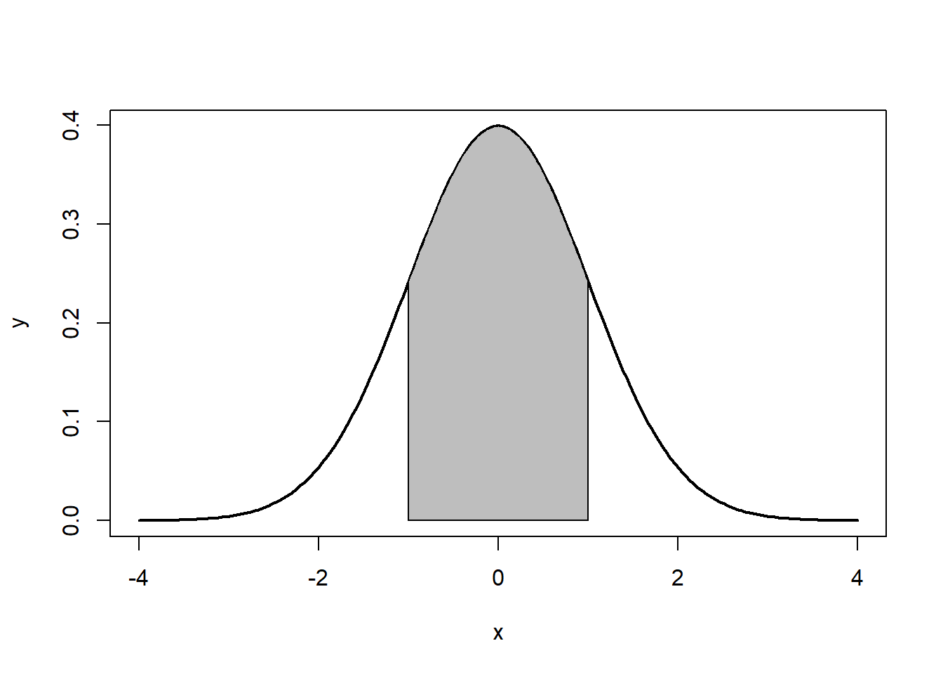
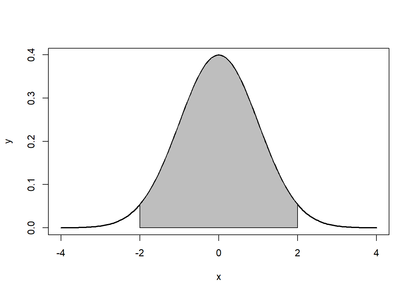
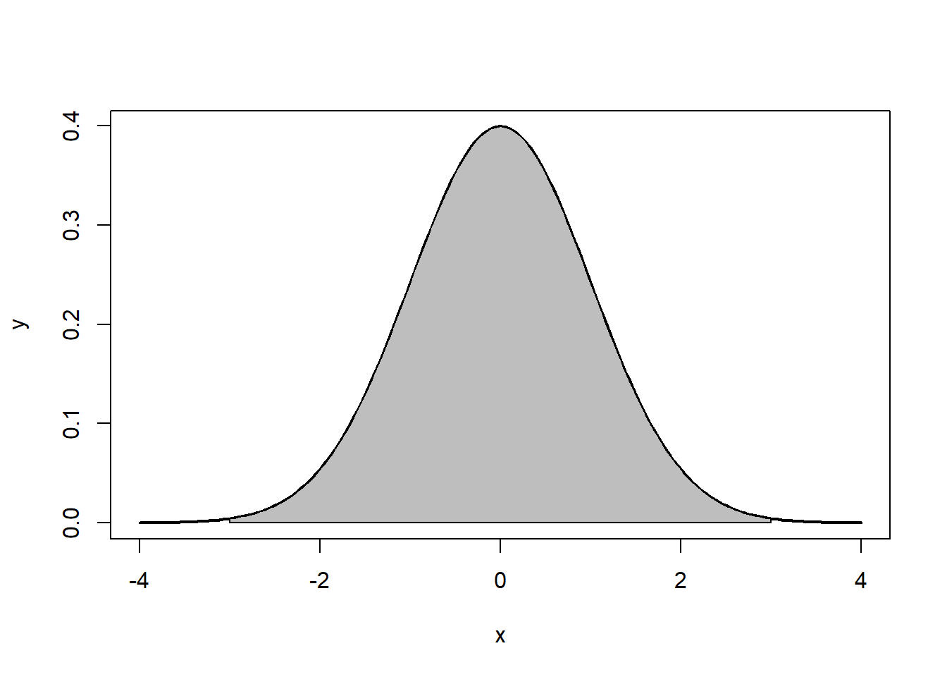
Note that the the tails go to ±∞±∞. In addition, the density of a distribution over the range of x is the key to hypothesis testing With a normal distribution, ∼68%∼68% of the observations will fall within 11 standard deviation of the mean, ∼95%∼95% will fall within 2 standard deviations, and ∼99.7%∼99.7% within 3 standard deviations. This is illustrated in Figures 5.2, 5.3, 5.4.
Figure \(\PageIndex{1}\): The Normal Distribution
Note that the the tails go to ±∞±∞. In addition, the density of a distribution over the range of x is the key to hypothesis testing With a normal distribution, ∼68%∼68% of the observations will fall within 11 standard deviation of the mean, ∼95%∼95% will fall within 2 standard deviations, and ∼99.7%∼99.7% within 3 standard deviations. This is illustrated in Figures 5.2, 5.3, 5.4.
For purposes of statistical inference, the normal distribution is one of the most important types of probability distributions. It forms the basis of many of the assumptions needed to do quantitative data analysis, and is the basis for a wide range of hypothesis tests. A standardized normal distribution has a mean, μμ, of 00 and a standard deviation (s.d.), σσ, of 11. The distribution of an outcome variable, YY, can be described:
Y∼N(μY,σ2Y)(5.1)(5.1)Y∼N(μY,σY2)
Where ∼∼ stands for “distributed as”, NN indicates the normal distribution, and mean μYμY and variance σ2YσY2 are the parameters. The probability function of the normal distribution is expressed below:
The Normal Probability Density Function: The probability density function (PDF) of a normal distribution with mean μμ and standard deviation σσ:
$f(x) = \frac{1}{\sigma \sqrt{2 \pi}} e^{-(x-\mu)^{2}/2\sigma^{2}}$The Standard Normal Probability Density Function: The standard normal PDF has a μ=0μ=0 and σ=1σ=1
$f(x) = \frac{1}{\sqrt{2 \pi}}e^{-x^{2}/2}$
Using the standard normal PDF, we can plot a normal distribution in R.
x <- seq(-4,4,length=200)
y <- 1/sqrt(2*pi)*exp(-x^2/2)
plot(x,y, type="l", lwd=2)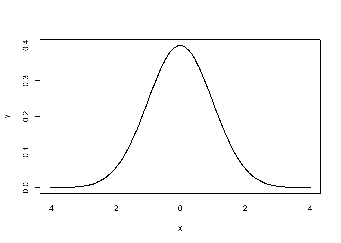
Note that the the tails go to ±∞±∞. In addition, the density of a distribution over the range of x is the key to hypothesis testing With a normal distribution, ∼68%∼68% of the observations will fall within 11 standard deviation of the mean, ∼95%∼95% will fall within 2 standard deviations, and ∼99.7%∼99.7% within 3 standard deviations. This is illustrated in Figures 5.2, 5.3, 5.4.
The normal distribution is characterized by several important properties. The distribution of observations is symmetrical around the mean μμ; the frequency of observations is highest (the mode) at μμ, with more extreme values occurring with lower frequency (this can be seen in Figure ??); and only the mean and variance are needed to characterize data and test simple hypotheses.
The Properties of the Normal Distribution
- It is symmetrical around its mean and median, μμ
- The highest probability (aka “the mode”) occurs at its mean value
- Extreme values occur in the tails
- It is fully described by its two parameters, μμ and σ2σ2
If the values for μμ and σ2σ2 are known, which might be the case with a population, then we can calculate a ZZ-score to compare differences in μμ and σ2σ2 between two normal distributions or obtain the probability for a given value given μμ and σ2σ2. The ZZ-score is calculated:
Z=Y−μYσ(5.2)(5.2)Z=Y−μYσ
Therefore, if we have a normal distribution with a μμ of 70 and a σ2σ2 of 9, we can calculate a probability for i=75i=75. First we calculate the ZZ-score, then we determine the probability of that score based on the normal distribution.
z <- (75-70)/3
z
## [1] 1.666667p <- pnorm(1.67)
p## [1] 0.9525403p <- 1-p
p## [1] 0.04745968As shown, a score of 7575 falls just outside two standard deviations (>0.95>0.95), and the probability of obtaining that score when μ=70μ=70 and σ2=9σ2=9 is just under 5%.
5.2.1 Standardizing a Normal Distribution and Z-scores
A distribution can be plotted using the raw scores found in the original data. That plot will have a mean and standard deviation calculated from the original data. To utilize the normal curve to determine probability functions and for inferential statistics we will want to convert that data so that it is standardized. We standardize so that the distribution is consistent across all distributions. That standardization produces a set of scores that have a mean of zero and a standard deviation of one. A standardized or Z-score of 1.5 means, therefore, that the score is one and a half standard deviations about the mean. A Z-score of -2.0 means that the score is two standard deviations below the mean.
As formula (4.4) indicated, standardizing is a simple process. To move the mean from its original value to a mean of zero, all you have to do is subtract the mean from each score. To standardize the standard deviation to one all that is necessary is to divide each score the standard deviation.
5.2.2 The Central Limit Theorem
An important property of samples is associated with the Central Limit Theorem (CLT). Imagine for a moment that we have a very large (or even infinite) population, from which we can draw as many samples as we’d like. According to the CLT, as the nn-size (number of observations) within a sample drawn from that population increases, the more the distribution of the means taken from samples of that size will resemble a normal distribution. This is illustrated in Figure \(\PageIndex{5}\). Also note that the population does not need to have a normal distribution for the CLT to apply. Finally, a distribution of means from a normal population will be approximately normal at any sample size.