1.3: Probability
- Page ID
- 1714
\( \newcommand{\vecs}[1]{\overset { \scriptstyle \rightharpoonup} {\mathbf{#1}} } \)
\( \newcommand{\vecd}[1]{\overset{-\!-\!\rightharpoonup}{\vphantom{a}\smash {#1}}} \)
\( \newcommand{\dsum}{\displaystyle\sum\limits} \)
\( \newcommand{\dint}{\displaystyle\int\limits} \)
\( \newcommand{\dlim}{\displaystyle\lim\limits} \)
\( \newcommand{\id}{\mathrm{id}}\) \( \newcommand{\Span}{\mathrm{span}}\)
( \newcommand{\kernel}{\mathrm{null}\,}\) \( \newcommand{\range}{\mathrm{range}\,}\)
\( \newcommand{\RealPart}{\mathrm{Re}}\) \( \newcommand{\ImaginaryPart}{\mathrm{Im}}\)
\( \newcommand{\Argument}{\mathrm{Arg}}\) \( \newcommand{\norm}[1]{\| #1 \|}\)
\( \newcommand{\inner}[2]{\langle #1, #2 \rangle}\)
\( \newcommand{\Span}{\mathrm{span}}\)
\( \newcommand{\id}{\mathrm{id}}\)
\( \newcommand{\Span}{\mathrm{span}}\)
\( \newcommand{\kernel}{\mathrm{null}\,}\)
\( \newcommand{\range}{\mathrm{range}\,}\)
\( \newcommand{\RealPart}{\mathrm{Re}}\)
\( \newcommand{\ImaginaryPart}{\mathrm{Im}}\)
\( \newcommand{\Argument}{\mathrm{Arg}}\)
\( \newcommand{\norm}[1]{\| #1 \|}\)
\( \newcommand{\inner}[2]{\langle #1, #2 \rangle}\)
\( \newcommand{\Span}{\mathrm{span}}\) \( \newcommand{\AA}{\unicode[.8,0]{x212B}}\)
\( \newcommand{\vectorA}[1]{\vec{#1}} % arrow\)
\( \newcommand{\vectorAt}[1]{\vec{\text{#1}}} % arrow\)
\( \newcommand{\vectorB}[1]{\overset { \scriptstyle \rightharpoonup} {\mathbf{#1}} } \)
\( \newcommand{\vectorC}[1]{\textbf{#1}} \)
\( \newcommand{\vectorD}[1]{\overrightarrow{#1}} \)
\( \newcommand{\vectorDt}[1]{\overrightarrow{\text{#1}}} \)
\( \newcommand{\vectE}[1]{\overset{-\!-\!\rightharpoonup}{\vphantom{a}\smash{\mathbf {#1}}}} \)
\( \newcommand{\vecs}[1]{\overset { \scriptstyle \rightharpoonup} {\mathbf{#1}} } \)
\(\newcommand{\longvect}{\overrightarrow}\)
\( \newcommand{\vecd}[1]{\overset{-\!-\!\rightharpoonup}{\vphantom{a}\smash {#1}}} \)
\(\newcommand{\avec}{\mathbf a}\) \(\newcommand{\bvec}{\mathbf b}\) \(\newcommand{\cvec}{\mathbf c}\) \(\newcommand{\dvec}{\mathbf d}\) \(\newcommand{\dtil}{\widetilde{\mathbf d}}\) \(\newcommand{\evec}{\mathbf e}\) \(\newcommand{\fvec}{\mathbf f}\) \(\newcommand{\nvec}{\mathbf n}\) \(\newcommand{\pvec}{\mathbf p}\) \(\newcommand{\qvec}{\mathbf q}\) \(\newcommand{\svec}{\mathbf s}\) \(\newcommand{\tvec}{\mathbf t}\) \(\newcommand{\uvec}{\mathbf u}\) \(\newcommand{\vvec}{\mathbf v}\) \(\newcommand{\wvec}{\mathbf w}\) \(\newcommand{\xvec}{\mathbf x}\) \(\newcommand{\yvec}{\mathbf y}\) \(\newcommand{\zvec}{\mathbf z}\) \(\newcommand{\rvec}{\mathbf r}\) \(\newcommand{\mvec}{\mathbf m}\) \(\newcommand{\zerovec}{\mathbf 0}\) \(\newcommand{\onevec}{\mathbf 1}\) \(\newcommand{\real}{\mathbb R}\) \(\newcommand{\twovec}[2]{\left[\begin{array}{r}#1 \\ #2 \end{array}\right]}\) \(\newcommand{\ctwovec}[2]{\left[\begin{array}{c}#1 \\ #2 \end{array}\right]}\) \(\newcommand{\threevec}[3]{\left[\begin{array}{r}#1 \\ #2 \\ #3 \end{array}\right]}\) \(\newcommand{\cthreevec}[3]{\left[\begin{array}{c}#1 \\ #2 \\ #3 \end{array}\right]}\) \(\newcommand{\fourvec}[4]{\left[\begin{array}{r}#1 \\ #2 \\ #3 \\ #4 \end{array}\right]}\) \(\newcommand{\cfourvec}[4]{\left[\begin{array}{c}#1 \\ #2 \\ #3 \\ #4 \end{array}\right]}\) \(\newcommand{\fivevec}[5]{\left[\begin{array}{r}#1 \\ #2 \\ #3 \\ #4 \\ #5 \\ \end{array}\right]}\) \(\newcommand{\cfivevec}[5]{\left[\begin{array}{c}#1 \\ #2 \\ #3 \\ #4 \\ #5 \\ \end{array}\right]}\) \(\newcommand{\mattwo}[4]{\left[\begin{array}{rr}#1 \amp #2 \\ #3 \amp #4 \\ \end{array}\right]}\) \(\newcommand{\laspan}[1]{\text{Span}\{#1\}}\) \(\newcommand{\bcal}{\cal B}\) \(\newcommand{\ccal}{\cal C}\) \(\newcommand{\scal}{\cal S}\) \(\newcommand{\wcal}{\cal W}\) \(\newcommand{\ecal}{\cal E}\) \(\newcommand{\coords}[2]{\left\{#1\right\}_{#2}}\) \(\newcommand{\gray}[1]{\color{gray}{#1}}\) \(\newcommand{\lgray}[1]{\color{lightgray}{#1}}\) \(\newcommand{\rank}{\operatorname{rank}}\) \(\newcommand{\row}{\text{Row}}\) \(\newcommand{\col}{\text{Col}}\) \(\renewcommand{\row}{\text{Row}}\) \(\newcommand{\nul}{\text{Nul}}\) \(\newcommand{\var}{\text{Var}}\) \(\newcommand{\corr}{\text{corr}}\) \(\newcommand{\len}[1]{\left|#1\right|}\) \(\newcommand{\bbar}{\overline{\bvec}}\) \(\newcommand{\bhat}{\widehat{\bvec}}\) \(\newcommand{\bperp}{\bvec^\perp}\) \(\newcommand{\xhat}{\widehat{\xvec}}\) \(\newcommand{\vhat}{\widehat{\vvec}}\) \(\newcommand{\uhat}{\widehat{\uvec}}\) \(\newcommand{\what}{\widehat{\wvec}}\) \(\newcommand{\Sighat}{\widehat{\Sigma}}\) \(\newcommand{\lt}{<}\) \(\newcommand{\gt}{>}\) \(\newcommand{\amp}{&}\) \(\definecolor{fillinmathshade}{gray}{0.9}\)Learning Objectives
- Simple rules about adding and multiplying probabilities
The basic idea of a statistical test is to identify a null hypothesis, collect some data, then estimate the probability of getting the observed data if the null hypothesis were true. If the probability of getting a result like the observed one is low under the null hypothesis, you conclude that the null hypothesis is probably not true. It is therefore useful to know a little about probability.
One way to think about probability is as the proportion of individuals in a population that have a particular characteristic. The probability of sampling a particular kind of individual is equal to the proportion of that kind of individual in the population. For example, in fall 2013 there were \(22,166\) students at the University of Delaware, and \(3,679\) of them were graduate students. If you sampled a single student at random, the probability that they would be a grad student would be \(\frac{3,679}{22,166}\) or \(0.166\). In other words, \(16.6\%\) of students were grad students, so if you'd picked one student at random, the probability that they were a grad student would have been \(16.6\%\).
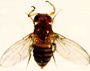
When dealing with probabilities in biology, you are often working with theoretical expectations, not population samples. For example, in a genetic cross of two individual Drosophila melanogaster that are heterozygous at the vestigial locus, Mendel's theory predicts that the probability of an offspring individual being a recessive homozygote (having teeny-tiny wings) is one-fourth, or \(0.25\). This is equivalent to saying that one-fourth of a population of offspring will have tiny wings.
Multiplying probabilities
You could take a semester-long course on mathematical probability, but most biologists just need to know a few basic principles. You calculate the probability that an individual has one value of a nominal variable AND another value of a second nominal variable by multiplying the probabilities of each value together.

For example, if the probability that a Drosophila in a cross has vestigial wings is one-fourth, AND the probability that it has legs where its antennae should be is three-fourths, the probability that it has vestigial wings AND leg-antennae is one-fourth times three-fourths, or \(0.25\times 0.75\), or \(0.1875\). This estimate assumes that the two values are independent, meaning that the probability of one value is not affected by the other value. In this case, independence would require that the two genetic loci were on different chromosomes, among other things.
Adding probabilities
The probability that an individual has one value OR another, MUTUALLY EXCLUSIVE, value is found by adding the probabilities of each value together. "Mutually exclusive" means that one individual could not have both values. For example, if the probability that a flower in a genetic cross is red is one-fourth, the probability that it is pink is one-half, and the probability that it is white is one-fourth, then the probability that it is red OR pink is one-fourth plus one-half, or three-fourths.
More complicated situations
When calculating the probability that an individual has one value OR another, and the two values are NOT MUTUALLY EXCLUSIVE, it is important to break things down into combinations that are mutually exclusive. For example, let's say you wanted to estimate the probability that a fly from the cross above had vestigial wings OR leg-antennae. You could calculate the probability for each of the four kinds of flies: normal wings/normal antennae (\(0.75\times 0.25=0.1875\)), normal wings/leg-antennae (\(0.75\times 0.75=0.5625\)), vestigial wings/normal antennae (\(0.25\times 0.25=0.0625\)), and vestigial wings/leg-antennae (\(0.25\times 0.75=0.1875\)). Then, since the last three kinds of flies are the ones with vestigial wings or leg-antennae, you'd add those probabilities up (\(0.5625+0.0625+0.1875=0.8125\)).
When to calculate probabilities
While there are some kind of probability calculations underlying all statistical tests, it is rare that you'll have to use the rules listed above. About the only time you'll actually calculate probabilities by adding and multiplying is when figuring out the expected values for a goodness-of-fit test.


