4.3: Large Sample Properties

Let $(X_t\colon t\in\mathbb{Z})$ be a weakly stationary time series with mean $\mu$, absolutely summable ACVF $\gamma(h)$ and spectral density $f(\omega)$. Proceeding as in the proof of Proposition4.2.2., one obtains

$$I(\omega_j)=\frac 1n\sum_{h={-n+1}}^{n-1}\sum_{t=1}^{n-|h|}(X_{t+|h|}-\mu)(X_t-\mu)\exp(-2\pi i\omega_jh), \label{Eq1}$$

provided $\omega_j\not=0$. Using this representation, the limiting behavior of the periodogram can be established.

Proposition 4.3.1

Let $I(\cdot)$ be the periodogram based on observations $X_1,\ldots,X_n$ of a weakly stationary process $(X_t\colon t\in\mathbb{Z})$, then, for any $\omega\not=0$,

$$E[I(\omega_{j:n})]\to f(\omega)\qquad(n\to\infty), \nonumber$$

where $\omega_{j:n}=j_n/n$ with $(j_n)_{n\in\mathbb{N}}$ chosen such that $\omega_{j:n}\to\omega$ as $n\to\infty$. If $\omega=0$, then

$$E[I(0)]-n\mu^2\to f(0)\qquad(n\to\infty). \nonumber$$

Proof. There are two limits involved in the computations of the periodogram mean. First, take the limit as $n\to\infty$. This, however, requires secondly that for each $n$ we have to work with a different set of Fourier frequencies. To adjust for this, we have introduced the notation $\omega_{j:n}$. If $\omega_j\not=0$ is a Fourier frequency ($n$ fixed!), then

$$E[I(\omega_j)]=\sum_{h=-n+1}^{n-1}\left(\frac{n-|h|}{n}\right)\gamma(h)\exp(-2\pi i\omega_jh). \nonumber$$

Therefore ($n\to\infty$!),

$$E[I(\omega_{j:n})]\to\sum_{h=-\infty}^\infty\gamma(h)\exp(-2\pi i\omega h)=f(\omega), \nonumber$$

thus proving the first claim. The second follows from $I(0)=n\bar{X}_n^2$ (see Proposition 4.2.2.), so that $E[I(0)]-n\mu^2=n(E[\bar{X}_n^2]-\mu^2)=n\mbox{Var}(\bar{X}_n) \to f(0)$ as $n\to\infty$ as in Chapter 2. The proof is complete.

Proposition 4.3.1. shows that the periodogram $I(\omega)$ is asymptotically unbiased for $f(\omega)$. It is, however, inconsistent. This is implied by the following proposition which is given without proof. It is not surprising considering that each value $I(\omega_j)$ is the sum of squares of only two random variables irrespective of the sample size.

Proposition 4.3.2.

If $(X_t\colon t\in\mathbb{Z})$ is a (causal or noncausal) weakly stationary time series such that

$$X_t=\sum_{j=-\infty}^\infty\psi_jZ_{t-j},\qquad t\in\mathbb{Z}, \nonumber$$

with $\sum_{j=-\infty}^\infty|\psi_j|<\infty and (Z_t)_{t\in\mathbb{Z}}\sim\mbox{WN}(0,\sigma^2)$, then

$$(\frac{2I(\omega_{1:n})}{f(\omega_1)},\ldots,\frac{2I(\omega_{m:n})}{f(\omega_m)}) \stackrel{\cal D}{\to}(\xi_1,\ldots,\xi_m), \nonumber$$

where $\omega_1,\ldots,\omega_m$ are $m$ distinct frequencies with $\omega_{j:n}\to\omega_j$ and $f(\omega_j)>0$. The variables $\xi_1,\ldots,\xi_m$ are independent, identical chi-squared distributed with two degrees of freedom.

The result of this proposition can be used to construct confidence intervals for the value of the spectral density at frequency $\omega$. To this end, denote by $\chi_2^2(\alpha)$ the lower tail probability of the chi-squared variable $\xi_j$, that is,

$$P(\xi_j\leq\chi_2^2(\alpha))=\alpha. \nonumber$$

Then, Proposition 4.3.2. implies that an approximate confidence interval with level $1-\alpha$ is given by

$$\frac{2I(\omega_{j:n})}{\chi_2^2(1-\alpha/2)}\leq f(\omega)\leq \frac{2I(\omega_{j:n})}{\chi_2^2(\alpha/2)}. \nonumber$$

Proposition 4.3.2. also suggests that confidence intervals can be derived simultaneously for several frequency components. Before confidence intervals are computed for the dominant frequency of the recruitment data return for a moment to the computation of the FFT which is the basis for the periodogram usage. To ensure a quick computation time, highly composite integers $n^\prime$ have to be used. To achieve this in general, the length of time series is adjusted by padding the original but detrended data by adding zeroes. In R, spectral analysis is performed with the function spec.pgram. To find out which $n^\prime$ is used for your particular data, type nextn(length(x)), assuming that your series is in x.

Figure 4.6: Averaged periodogram of the recruitment data discussed in Example 4.3.1.

Example 4.3.1.

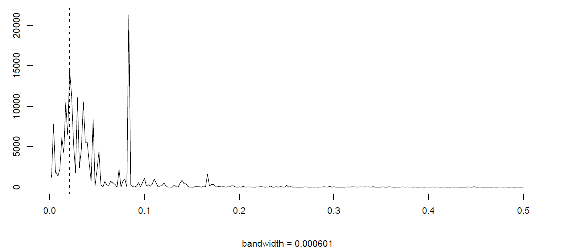
Figure 4.5 displays the periodogram of the recruitment data which has been discussed in Example 3.3.5. It shows a strong annual frequency component at $\omega=1/12$ as well as several spikes in the neighborhood of the El Ni$\tilde{n}$o frequency $\omega=1/48$. Higher frequency components with $\omega>.3$ are virtually absent. Even though an AR(2) model was fitted to this data in Chapter 3 to produce future values based on this fit, it is seen that the periodogram here does not validate this fit as the spectral density of an AR(2) process (as computed in Example 4.2.3.) is qualitatively different. In R, the following commands can be used (nextn(length(rec)) gives $n^\prime=480$ here if the recruitment data is stored in rec as before).

>rec.pgram=spec.pgram(rec, taper=0, log="no")

>abline(v=1/12, lty=2)

>abline(v=1/48, lty=2)

The function spec.pgram allows you to fine-tune the spectral analysis. For our purposes, we always use the specifications given above for the raw periodogram (taper allows you, for example, to exclusively look at a particular frequency band, log allows you to plot the log-periodogram and is the R standard).

To compute the confidence intervals for the two dominating frequencies $1/12$ and $1/48$, you can use the following R code, noting that $1/12=40/480$ and $1/48=10/480$.

>rec.pgram{\$}spec[40]

[1] 21332.94

>rec.pgram{\$}spec[10]

[1] 14368.42

>u=qchisq(.025, 2); l=qchisq(.975, 2)

>2*rec.pgram{\$}spec[40]/l

>2*rec.pgram{\$}spec[40]/u

>2*rec.pgram{\$}spec[10]/l

~2*rec.pgram{\$}spec[10]/u

Using the numerical values of this analysis, the following confidence intervals are obtained at the level $\alpha=.1$:

$$f(1/12)\in(5783.041,842606.2)\qquad\mbox{and}\qquad f(1/48)\in(3895.065, 567522.5). \nonumber$$

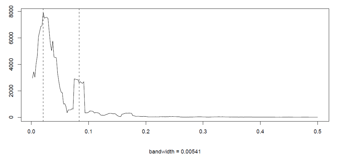
These are much too wide and alternatives to the raw periodogram are needed. These are provided, for example, by a smoothing approach which uses an averaging procedure over a band of neighboring frequencies. This can be done as follows.

>k=kernel("daniell",4)

>rec.ave=spec.pgram(rec, k, taper=0, log="no")

> abline(v=1/12, lty=2)

> abline(v=1/48, lty=2)

> rec.ave$bandwidth

[1] 0.005412659\medskip

The resulting smoothed periodogram is shown in Figure 4.6. It is less noisy, as is expected from taking averages. More precisely, a two-sided Daniell filter with $m=4$ was used here with $L=2m+1$ neighboring frequencies

$$\omega_k=\omega_j+\frac kn,\qquad k=-m,\ldots,m, \nonumber$$

to compute the periodogram at $\omega_j=j/n$. The resulting plot in Figure 4.6 shows, on the other hand, that the sharp annual peak has been flattened considerably. The bandwidth reported in R can be computed as $b=L/(\sqrt{12}n)$. To compute confidence intervals one has to adjust the previously derived formula. This is done by taking changing the degrees of freedom from 2 to $df=2Ln/n^\prime$ (if the zeroes where appended) and leads to

$$\frac{df}{\chi^2_{df}(1-\alpha/2)} \sum_{k=-m}^mf(\omega_j+\frac kn) \leq f(\omega) \leq \frac{df}{\chi^2_{df}(\alpha/2)}\sum_{k=-m}^mf(\omega_j+\frac kn) \nonumber$$

for $\omega\approx\omega_j$. For the recruitment data the following R code can be used:

>df=ceiling(rec.ave{\$}df)

>u=qchisq(.025,df), l~=~qchisq(.975,df)

>df*rec.ave{\$}spec[40]/l

>df*rec.ave{\$}spec[40]/u

>df*rec.ave{\$}spec[10]/l

>df*rec.ave{\$}spec[10]/u

Figure 4.7: The modified Daniell periodogram of the recruitment data discussed in Example 4.3.1.

to get the confidence intervals

$$f(1/12)\in(1482.427, 5916.823)\qquad\mbox{and}\qquad f(1/48)\in(4452.583, 17771.64). \nonumber$$

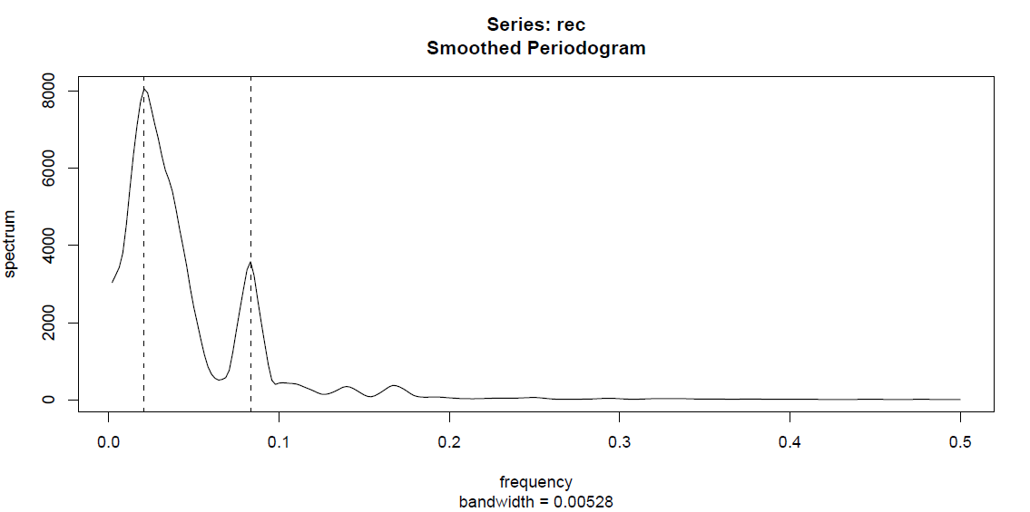
The compromise between the noisy raw periodogram and further smoothing as described here (with $L=9$) reverses the magnitude of the $1/12$ annual frequency and the $1/48$ El Ni$\tilde{n}$o component. This is due to the fact that the annual peak is a very sharp one, with neighboring frequencies being basically zero. For the $1/48$ component, there are is a whole band of neighboring frequency which also contribute the El Ni$\tilde{n}$o phenomenon is irregular and does only on average appear every four years). Moreover, the annual cycle is now distributed over a whole range. One way around this issue is provided by the use of other kernels such as the modified Daniell kernel given in R as kernel("modified.daniell", c(3,3)). This leads to the spectral density in Figure 4.7.

Contributers

• Alexander Aue (Department of Statistics, University of California, Davis)

• Integrated by Brett Nakano (statistics, UC Davis)

Demo: I really love the way that Equation $\ref{Eq1}$ looks.