3.9: Putting It All Together- SD and 3 M's
- Page ID
- 17323
\( \newcommand{\vecs}[1]{\overset { \scriptstyle \rightharpoonup} {\mathbf{#1}} } \)
\( \newcommand{\vecd}[1]{\overset{-\!-\!\rightharpoonup}{\vphantom{a}\smash {#1}}} \)
\( \newcommand{\id}{\mathrm{id}}\) \( \newcommand{\Span}{\mathrm{span}}\)
( \newcommand{\kernel}{\mathrm{null}\,}\) \( \newcommand{\range}{\mathrm{range}\,}\)
\( \newcommand{\RealPart}{\mathrm{Re}}\) \( \newcommand{\ImaginaryPart}{\mathrm{Im}}\)
\( \newcommand{\Argument}{\mathrm{Arg}}\) \( \newcommand{\norm}[1]{\| #1 \|}\)
\( \newcommand{\inner}[2]{\langle #1, #2 \rangle}\)
\( \newcommand{\Span}{\mathrm{span}}\)
\( \newcommand{\id}{\mathrm{id}}\)
\( \newcommand{\Span}{\mathrm{span}}\)
\( \newcommand{\kernel}{\mathrm{null}\,}\)
\( \newcommand{\range}{\mathrm{range}\,}\)
\( \newcommand{\RealPart}{\mathrm{Re}}\)
\( \newcommand{\ImaginaryPart}{\mathrm{Im}}\)
\( \newcommand{\Argument}{\mathrm{Arg}}\)
\( \newcommand{\norm}[1]{\| #1 \|}\)
\( \newcommand{\inner}[2]{\langle #1, #2 \rangle}\)
\( \newcommand{\Span}{\mathrm{span}}\) \( \newcommand{\AA}{\unicode[.8,0]{x212B}}\)
\( \newcommand{\vectorA}[1]{\vec{#1}} % arrow\)
\( \newcommand{\vectorAt}[1]{\vec{\text{#1}}} % arrow\)
\( \newcommand{\vectorB}[1]{\overset { \scriptstyle \rightharpoonup} {\mathbf{#1}} } \)
\( \newcommand{\vectorC}[1]{\textbf{#1}} \)
\( \newcommand{\vectorD}[1]{\overrightarrow{#1}} \)
\( \newcommand{\vectorDt}[1]{\overrightarrow{\text{#1}}} \)
\( \newcommand{\vectE}[1]{\overset{-\!-\!\rightharpoonup}{\vphantom{a}\smash{\mathbf {#1}}}} \)
\( \newcommand{\vecs}[1]{\overset { \scriptstyle \rightharpoonup} {\mathbf{#1}} } \)
\( \newcommand{\vecd}[1]{\overset{-\!-\!\rightharpoonup}{\vphantom{a}\smash {#1}}} \)
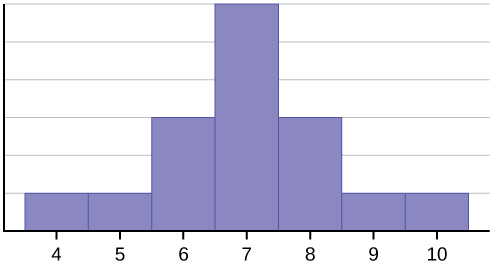
\(\newcommand{\avec}{\mathbf a}\) \(\newcommand{\bvec}{\mathbf b}\) \(\newcommand{\cvec}{\mathbf c}\) \(\newcommand{\dvec}{\mathbf d}\) \(\newcommand{\dtil}{\widetilde{\mathbf d}}\) \(\newcommand{\evec}{\mathbf e}\) \(\newcommand{\fvec}{\mathbf f}\) \(\newcommand{\nvec}{\mathbf n}\) \(\newcommand{\pvec}{\mathbf p}\) \(\newcommand{\qvec}{\mathbf q}\) \(\newcommand{\svec}{\mathbf s}\) \(\newcommand{\tvec}{\mathbf t}\) \(\newcommand{\uvec}{\mathbf u}\) \(\newcommand{\vvec}{\mathbf v}\) \(\newcommand{\wvec}{\mathbf w}\) \(\newcommand{\xvec}{\mathbf x}\) \(\newcommand{\yvec}{\mathbf y}\) \(\newcommand{\zvec}{\mathbf z}\) \(\newcommand{\rvec}{\mathbf r}\) \(\newcommand{\mvec}{\mathbf m}\) \(\newcommand{\zerovec}{\mathbf 0}\) \(\newcommand{\onevec}{\mathbf 1}\) \(\newcommand{\real}{\mathbb R}\) \(\newcommand{\twovec}[2]{\left[\begin{array}{r}#1 \\ #2 \end{array}\right]}\) \(\newcommand{\ctwovec}[2]{\left[\begin{array}{c}#1 \\ #2 \end{array}\right]}\) \(\newcommand{\threevec}[3]{\left[\begin{array}{r}#1 \\ #2 \\ #3 \end{array}\right]}\) \(\newcommand{\cthreevec}[3]{\left[\begin{array}{c}#1 \\ #2 \\ #3 \end{array}\right]}\) \(\newcommand{\fourvec}[4]{\left[\begin{array}{r}#1 \\ #2 \\ #3 \\ #4 \end{array}\right]}\) \(\newcommand{\cfourvec}[4]{\left[\begin{array}{c}#1 \\ #2 \\ #3 \\ #4 \end{array}\right]}\) \(\newcommand{\fivevec}[5]{\left[\begin{array}{r}#1 \\ #2 \\ #3 \\ #4 \\ #5 \\ \end{array}\right]}\) \(\newcommand{\cfivevec}[5]{\left[\begin{array}{c}#1 \\ #2 \\ #3 \\ #4 \\ #5 \\ \end{array}\right]}\) \(\newcommand{\mattwo}[4]{\left[\begin{array}{rr}#1 \amp #2 \\ #3 \amp #4 \\ \end{array}\right]}\) \(\newcommand{\laspan}[1]{\text{Span}\{#1\}}\) \(\newcommand{\bcal}{\cal B}\) \(\newcommand{\ccal}{\cal C}\) \(\newcommand{\scal}{\cal S}\) \(\newcommand{\wcal}{\cal W}\) \(\newcommand{\ecal}{\cal E}\) \(\newcommand{\coords}[2]{\left\{#1\right\}_{#2}}\) \(\newcommand{\gray}[1]{\color{gray}{#1}}\) \(\newcommand{\lgray}[1]{\color{lightgray}{#1}}\) \(\newcommand{\rank}{\operatorname{rank}}\) \(\newcommand{\row}{\text{Row}}\) \(\newcommand{\col}{\text{Col}}\) \(\renewcommand{\row}{\text{Row}}\) \(\newcommand{\nul}{\text{Nul}}\) \(\newcommand{\var}{\text{Var}}\) \(\newcommand{\corr}{\text{corr}}\) \(\newcommand{\len}[1]{\left|#1\right|}\) \(\newcommand{\bbar}{\overline{\bvec}}\) \(\newcommand{\bhat}{\widehat{\bvec}}\) \(\newcommand{\bperp}{\bvec^\perp}\) \(\newcommand{\xhat}{\widehat{\xvec}}\) \(\newcommand{\vhat}{\widehat{\vvec}}\) \(\newcommand{\uhat}{\widehat{\uvec}}\) \(\newcommand{\what}{\widehat{\wvec}}\) \(\newcommand{\Sighat}{\widehat{\Sigma}}\) \(\newcommand{\lt}{<}\) \(\newcommand{\gt}{>}\) \(\newcommand{\amp}{&}\) \(\definecolor{fillinmathshade}{gray}{0.9}\)Consider the histogram of a frequency distribution in Figure \(\PageIndex{1}\).

The histogram displays a symmetrical distribution of data. A distribution is symmetrical if a vertical line can be drawn at some point in the histogram such that the shape to the left and the right of the vertical line are mirror images of each other. The mean, the median, and the mode are each seven for these data. In a perfectly symmetrical distribution, the mean and the median are the same. This example has one mode (unimodal), and the mode is the same as the mean and median. In a symmetrical distribution that has two modes (bimodal), the two modes would be different from the mean and median.
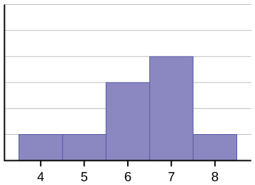
The histogram for the data in Figure \(\PageIndex{2}\) is not symmetrical. The right-hand side seems "chopped off" compared to the left side. A distribution of this type is called negatively skewed because the tail is pulled out to the left.

Exercise \(\PageIndex{1}\)
The data used to create Figure \(\PageIndex{2}\) is: 4, 5, 6, 6, 6, 7, 7, 7, 7, and 8. What is the mean? What is the median? What is the mode?
- Answer
-
The mean is 6.3. The median is 6.5. The mode is 7.
(We cannnot include units in these because this is example data; we don't know what was measured.)
Notice that the mean is less than the median, and they are both less than the mode. Distributions of data are negatively skewed when the mean is lower than the median. The extreme low scores bring the mean down, but their extremeity doesn't affect the median (or mode).
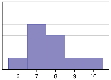
The histogram in Figure \(\PageIndex{3}\) is also not symmetrical, but is positively skewed as the tail points to the right.

Exercise \(\PageIndex{3}\)
The data used to create Figure \(\PageIndex{3}\) is: 6, 7, 7, 7, 7, 8, 8, 8, 9, and 10. What is the mean? What is the median? What is the mode?
- Answer
-
The mean is 7.7. The median is 7.5. The mode is 7.
(We cannnot include units in these because this is example data; we don't know what was measured.)
In contrast to the negatively skewed distribution in Figure \(\PageIndex{2}\), the positively skewed distribution's mean is larger than the median. Looking at Figure \(\PageIndex{3}\), you can see how the few high scores pulled the mean up, but extreme scores do not affect what number is in the middle (the median).
Generally, if the distribution of data is skewed to the left, the mean is less than the median, which is often less than the mode. If the distribution of data is skewed to the right, the mode is often less than the median, which is less than the mean.
Skewness and symmetry become important when we discuss probability distributions in later chapters.
Note
Do you think that is bigger in the symmetrical distribution shown in Figure \(\PageIndex{1}\) or the skewed distribution in Figure \(\PageIndex{2}\)? Let's see!
First, let's work together to practice calculating a standard deviation using the data from Figure \(\PageIndex{1}\).
Example \(\PageIndex{1}\)
The data from Figure \(\PageIndex{1}\) is in Table \(\PageIndex{1}\). Use the table to find the Sum of Squares, then finish the standard deviation formula for a sample.
Solution
| \(\mathrm{X}\) | \(X-\overline{X}\) | Sums of Squares (\((X-\overline {X})^{2}\)) |
|---|---|---|
| 4 | \(4-\overline{X} = -3 \) | \((X-\overline {X})^{2} = -3^{2} = 9 \) |
| 5 | \(5-\overline{X} = -2 \) | \((X-\overline {X})^{2} = -2^{2} = 4 \) |
| 6 | \(6-\overline{X} = -1 \) | \((X-\overline {X})^{2} = -1^{2} = 1 \) |
| 6 | \(6-\overline{X} = -1 \) | \((X-\overline {X})^{2} = -1^{2} = 1 \) |
| 6 | \(6-\overline{X} = -1 \) | \((X-\overline {X})^{2} = -1^{2} = 1 \) |
| 7 | \(7-\overline{X} = -0 \) | \((X-\overline {X})^{2} = 0^{2} = 0 \) |
| 7 | \(7-\overline{X} = -0 \) | \((X-\overline {X})^{2} = 0^{2} = 0 \) |
| 7 | \(7-\overline{X} = -0 \) | \((X-\overline {X})^{2} = 0^{2} = 0 \) |
| 7 | \(7-\overline{X} = -0 \) | \((X-\overline {X})^{2} = 0^{2} = 0 \) |
| 7 | \(7-\overline{X} = -0 \) | \((X-\overline {X})^{2} = 0^{2} = 0 \) |
| 7 | \(7-\overline{X} = -0 \) | \((X-\overline {X})^{2} = 0^{2} = 0 \) |
| 8 | \(8-\overline{X} = 1 \) | \((X-\overline {X})^{2} = 1^{2} = 1 \) |
| 8 | \(8-\overline{X} = 1 \) | \((X-\overline {X})^{2} = 1^{2} = 1 \) |
| 8 | \(8-\overline{X} = 1 \) | \((X-\overline {X})^{2} = 1^{2} = 1 \) |
| 9 | \(9-\overline{X} = 2 \) | \((X-\overline {X})^{2} = 2^{2} = 4 \) |
| 10 | \(10-\overline{X} = 3 \) | \((X-\overline {X})^{2} = 3^{2} = 9 \) |
| \(\Sigma = 112\) | \(\Sigma = 0\) | \(\Sigma = 32\) |
The last column (the one on the right) is the squared deviations. So, when they are summed to 32, you have the Sum of Squares.
\[s= \sqrt{\dfrac{S S}{d f}} = \sqrt{\dfrac{\sum(X-\overline {X})^{2}}{N-1}} \nonumber \]
As this suggests, you then divide the Sum of Squares by N-1 (N is the number of scores), so:
\[{N-1} = 16-1 = 15 \nonumber \]
Then,
\[s= \sqrt{\dfrac{S S}{d f}} = \sqrt{\dfrac{\sum(X-\overline {X})^{2}}{N-1}} = \dfrac{32}{15} = 2.1\overline3 \nonumber \]
And the final step of square rooting to get it back into whatever units we started with:
\[s= \sqrt{\dfrac{S S}{d f}} = \sqrt{\dfrac{\sum(X-\overline {X})^{2}}{N-1}} = \sqrt{2.1\overline3} = 1.460593 \nonumber \]
The standard deviation of the data from Figure \(\PageIndex{1}\) is 1.46!
Now, try it on your own!
Exercise \(\PageIndex{2}\)
Compute a standard deviation with the data from Figure \(\PageIndex{2}\) that is in Table \(\PageIndex{2}\).
| \(\mathrm{X}\) | \(X-\overline{X}\) | Sums of Squares (\((X-\overline {X})^{2}\)) |
|---|---|---|
| 4 | ||
| 5 | ||
| 6 | ||
| 6 | ||
| 6 | ||
| 7 | ||
| 7 | ||
| 7 | ||
| 7 | ||
| 8 | ||
| \(\Sigma = 63\) | \(\Sigma = 0\) | \(\Sigma = ?\) |
\[s= \sqrt{\dfrac{S S}{d f}} = \sqrt{\dfrac{\sum(X-\overline {X})^{2}}{N-1}} \nonumber \]
- Answer
-
The standard deviation for the data from Figure \(\PageIndex{2}\) is 1.16 (rounded from 1.159502).
If you didn't get something close to this, check that you used the correct N (number of scores) fo 10 in this sample. Another thing to check is that your Sum of Squares should be 12.1; often, simple adding or messing up the mean will wreck the rest of your calculations!
So what did we learn from Example \(\PageIndex{1}\) and Exercise \(\PageIndex{2}\)? The skewed distribution had a smaller standard deviation than the symmetrical distribution. Why might that be? Maybe looking at the range will help? The range of the symmetrical distribution was 6 (\(10 - 4 = 6 \)), while the range of the skewed distribution was 4. Having a smaller range means that there was no extreme scores, so that could explain the lower standard deviation.
Quiz Yourself!
You can use the following to text yourself to see if you understand the relationships between the measures of central tendency (mean, median, and mode) and th measures of variability (range and standard deviation) in relation to the shape of distributions of data.
Exercise \(\PageIndex{3}\)
When the data are symmetrical, what is the typical relationship between the mean and median?
Answer
When the data are symmetrical, the mean and median are close or the same.
Exercise \(\PageIndex{4}\)
Describe the shape of this distribution.

Answer
The distribution is skewed right because it looks pulled out to the right.
Exercise \(\PageIndex{5}\)
Describe the relationship between the mode and the median of this distribution.

Answer
The mode and the median are the same. In this case, they are both five.
Exercise \(\PageIndex{6}\)
Describe the shape of this distribution.

Answer
The distribution is skewed left because it looks pulled out to the left.
Exercise \(\PageIndex{7}\)
Which is the greatest, the mean, the mode, or the median of the data set?
11; 11; 12; 12; 12; 12; 13; 15; 17; 22; 22; 22
Answer
The mode is 12, the median is 12.5, and the mean is 15.1. The mean is the largest.
Putting It All Together: SD & 3 M's
Let's look at everything that we know about the data for Figure \(\PageIndex{2}\).
First, we know the measures of central tendency. These tells us where the "center" of the distribution might be. For Figure \(\PageIndex{2}\), the sample mean was 6.3, the median was 6.5, and the mode was 7. This suggests that the center of the distribution of data was probably somewhere between 6.3 and 7. Even without seeing the histogram, I might think that the distribution was skewed because the mean was smaller than the median. It wasn't that much smaller (0.2), so I wouldn't bet my life on that one.
Second, we know some measures of variability. The range is 4 (the highest score of 8 minus the lowest score of 4), and the standard deviation was 1.16. Compared to a mean of 6.3, a standard deviation of 1.16 might be considered medium or slightly large. A medium standard deviation would suggest a bell-shaped curve, while a larger standard deviation would suggest a wide and flat distribution or a skewed distribution.
Finally, I can look at the actual Figure \(\PageIndex{2}\). That shows a negatively skewed distribution. I can find where the mode, median, and mean would be on Figure \(\PageIndex{2}\), and look to see what scores might fall within one standard deviation above and below the mean.
Contributors and Attributions
Barbara Illowsky and Susan Dean (De Anza College) with many other contributing authors. Content produced by OpenStax College is licensed under a Creative Commons Attribution License 4.0 license. Download for free at http://cnx.org/contents/30189442-699...b91b9de@18.114.
- Dr. MO (Taft College)


