
Glossary
- Page ID
- 22185
\( \newcommand{\vecs}[1]{\overset { \scriptstyle \rightharpoonup} {\mathbf{#1}} } \)
\( \newcommand{\vecd}[1]{\overset{-\!-\!\rightharpoonup}{\vphantom{a}\smash {#1}}} \)
\( \newcommand{\id}{\mathrm{id}}\) \( \newcommand{\Span}{\mathrm{span}}\)
( \newcommand{\kernel}{\mathrm{null}\,}\) \( \newcommand{\range}{\mathrm{range}\,}\)
\( \newcommand{\RealPart}{\mathrm{Re}}\) \( \newcommand{\ImaginaryPart}{\mathrm{Im}}\)
\( \newcommand{\Argument}{\mathrm{Arg}}\) \( \newcommand{\norm}[1]{\| #1 \|}\)
\( \newcommand{\inner}[2]{\langle #1, #2 \rangle}\)
\( \newcommand{\Span}{\mathrm{span}}\)
\( \newcommand{\id}{\mathrm{id}}\)
\( \newcommand{\Span}{\mathrm{span}}\)
\( \newcommand{\kernel}{\mathrm{null}\,}\)
\( \newcommand{\range}{\mathrm{range}\,}\)
\( \newcommand{\RealPart}{\mathrm{Re}}\)
\( \newcommand{\ImaginaryPart}{\mathrm{Im}}\)
\( \newcommand{\Argument}{\mathrm{Arg}}\)
\( \newcommand{\norm}[1]{\| #1 \|}\)
\( \newcommand{\inner}[2]{\langle #1, #2 \rangle}\)
\( \newcommand{\Span}{\mathrm{span}}\) \( \newcommand{\AA}{\unicode[.8,0]{x212B}}\)
\( \newcommand{\vectorA}[1]{\vec{#1}} % arrow\)
\( \newcommand{\vectorAt}[1]{\vec{\text{#1}}} % arrow\)
\( \newcommand{\vectorB}[1]{\overset { \scriptstyle \rightharpoonup} {\mathbf{#1}} } \)
\( \newcommand{\vectorC}[1]{\textbf{#1}} \)
\( \newcommand{\vectorD}[1]{\overrightarrow{#1}} \)
\( \newcommand{\vectorDt}[1]{\overrightarrow{\text{#1}}} \)
\( \newcommand{\vectE}[1]{\overset{-\!-\!\rightharpoonup}{\vphantom{a}\smash{\mathbf {#1}}}} \)
\( \newcommand{\vecs}[1]{\overset { \scriptstyle \rightharpoonup} {\mathbf{#1}} } \)
\( \newcommand{\vecd}[1]{\overset{-\!-\!\rightharpoonup}{\vphantom{a}\smash {#1}}} \)
\(\newcommand{\avec}{\mathbf a}\) \(\newcommand{\bvec}{\mathbf b}\) \(\newcommand{\cvec}{\mathbf c}\) \(\newcommand{\dvec}{\mathbf d}\) \(\newcommand{\dtil}{\widetilde{\mathbf d}}\) \(\newcommand{\evec}{\mathbf e}\) \(\newcommand{\fvec}{\mathbf f}\) \(\newcommand{\nvec}{\mathbf n}\) \(\newcommand{\pvec}{\mathbf p}\) \(\newcommand{\qvec}{\mathbf q}\) \(\newcommand{\svec}{\mathbf s}\) \(\newcommand{\tvec}{\mathbf t}\) \(\newcommand{\uvec}{\mathbf u}\) \(\newcommand{\vvec}{\mathbf v}\) \(\newcommand{\wvec}{\mathbf w}\) \(\newcommand{\xvec}{\mathbf x}\) \(\newcommand{\yvec}{\mathbf y}\) \(\newcommand{\zvec}{\mathbf z}\) \(\newcommand{\rvec}{\mathbf r}\) \(\newcommand{\mvec}{\mathbf m}\) \(\newcommand{\zerovec}{\mathbf 0}\) \(\newcommand{\onevec}{\mathbf 1}\) \(\newcommand{\real}{\mathbb R}\) \(\newcommand{\twovec}[2]{\left[\begin{array}{r}#1 \\ #2 \end{array}\right]}\) \(\newcommand{\ctwovec}[2]{\left[\begin{array}{c}#1 \\ #2 \end{array}\right]}\) \(\newcommand{\threevec}[3]{\left[\begin{array}{r}#1 \\ #2 \\ #3 \end{array}\right]}\) \(\newcommand{\cthreevec}[3]{\left[\begin{array}{c}#1 \\ #2 \\ #3 \end{array}\right]}\) \(\newcommand{\fourvec}[4]{\left[\begin{array}{r}#1 \\ #2 \\ #3 \\ #4 \end{array}\right]}\) \(\newcommand{\cfourvec}[4]{\left[\begin{array}{c}#1 \\ #2 \\ #3 \\ #4 \end{array}\right]}\) \(\newcommand{\fivevec}[5]{\left[\begin{array}{r}#1 \\ #2 \\ #3 \\ #4 \\ #5 \\ \end{array}\right]}\) \(\newcommand{\cfivevec}[5]{\left[\begin{array}{c}#1 \\ #2 \\ #3 \\ #4 \\ #5 \\ \end{array}\right]}\) \(\newcommand{\mattwo}[4]{\left[\begin{array}{rr}#1 \amp #2 \\ #3 \amp #4 \\ \end{array}\right]}\) \(\newcommand{\laspan}[1]{\text{Span}\{#1\}}\) \(\newcommand{\bcal}{\cal B}\) \(\newcommand{\ccal}{\cal C}\) \(\newcommand{\scal}{\cal S}\) \(\newcommand{\wcal}{\cal W}\) \(\newcommand{\ecal}{\cal E}\) \(\newcommand{\coords}[2]{\left\{#1\right\}_{#2}}\) \(\newcommand{\gray}[1]{\color{gray}{#1}}\) \(\newcommand{\lgray}[1]{\color{lightgray}{#1}}\) \(\newcommand{\rank}{\operatorname{rank}}\) \(\newcommand{\row}{\text{Row}}\) \(\newcommand{\col}{\text{Col}}\) \(\renewcommand{\row}{\text{Row}}\) \(\newcommand{\nul}{\text{Nul}}\) \(\newcommand{\var}{\text{Var}}\) \(\newcommand{\corr}{\text{corr}}\) \(\newcommand{\len}[1]{\left|#1\right|}\) \(\newcommand{\bbar}{\overline{\bvec}}\) \(\newcommand{\bhat}{\widehat{\bvec}}\) \(\newcommand{\bperp}{\bvec^\perp}\) \(\newcommand{\xhat}{\widehat{\xvec}}\) \(\newcommand{\vhat}{\widehat{\vvec}}\) \(\newcommand{\uhat}{\widehat{\uvec}}\) \(\newcommand{\what}{\widehat{\wvec}}\) \(\newcommand{\Sighat}{\widehat{\Sigma}}\) \(\newcommand{\lt}{<}\) \(\newcommand{\gt}{>}\) \(\newcommand{\amp}{&}\) \(\definecolor{fillinmathshade}{gray}{0.9}\)| Words (or words that have the same definition) | The definition is case sensitive | (Optional) Image to display with the definition [Not displayed in Glossary, only in pop-up on pages] | (Optional) Caption for Image | (Optional) External or Internal Link | (Optional) Source for Definition |
|---|---|---|---|---|---|
| (Eg. "Genetic, Hereditary, DNA ...") | (Eg. "Relating to genes or heredity") |  |
The infamous double helix | https://bio.libretexts.org/ | CC-BY-SA; Delmar Larsen |
| Word(s) | Definition | Image | Caption | Link | Source |
|---|---|---|---|---|---|
| Statistical analysis, statistical analyses | Procedures to organize and interpret numerical information | CC-BY Michelle Oja | |||
| Statistic | The results of statistical analyses | CC-BY Michelle Oja | |||
| Independent Variable, IV | The variable that the researcher thinks is the cause of the effect (the DV). The IV is sometimes also called a "predictor" or "predicting variable". | CC-BY Michelle Oja | |||
| Dependent Variable, DV | The variable that you think is the effect (the thing that the IV changes). The DV is the outcome variable, the thing that you want to improve. | CC-BY Michelle Oja | |||
| Sample, samples | People who participate in a study; the smaller group that the data is gathered from. | CC-BY Michelle Oja | |||
| Population | The biggest group that your sample can represent. | CC-BY Michelle Oja | |||
| Ratio | True numerical scale of measurement; type of variable that is measured, and zero means that there is none of it. | CC-BY Michelle Oja | |||
| Interval | Created numerical scale of measurement; type of variable that is measured, and the intervals between each measurement are equal (but zero does not mean the absence of the measured item). | CC-BY Michelle Oja | |||
| Ordinal | Scale of measurement in which levels have an order; a type of variable that can be put in numerical order. The variables are in ranks (first, second, third, etc.). | CC-BY Michelle Oja | |||
| Nominal | Scale of measurement that names the variable's levels; type of variable that has a quality or name, but not a number that means something. | CC-BY Michelle Oja | |||
| Quantitative variable, quantitative variables | Type of variable that is measured with some sort of scale that uses numbers that measure something. | CC-BY Michelle Oja | |||
| Qualitative variable, qualitative variables | Type of variable that has different values to represent different categories or kinds This is the same as the nominal scale of measurement. | CC-BY Michelle Oja | |||
| Frequency Table | Table showing each score in the “x” column, and how many people earned that score in the “f” column. The “x” stands in for whatever the score is, and the “f” stands for frequency. | CC-BY Michelle Oja | |||
| Outlier | An extreme score, a score that seems much higher or much lower than most of the other scores (There is a technical way to calculate whether a score is an outlier or not, but you don't need to know it.) | CC-BY Michelle Oja | |||
| Skew, skewed distribution | A distribution in which many scores are bunched up to one side, and there are only a few scores on the other side. | CC-BY Michelle Oja | |||
| Positive skew | The scores are bunched to the left, and the thin tail is pointing to the right. | 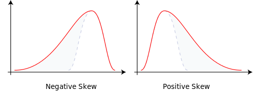.png?revision=1) |
Positive skew is shown on the right panel. | Rodolfo Hermans (Godot), CC BY-SA 3.0 via Wikimedia Commons | CC-BY Michelle Oja |
| Negative skew | The scores are bunched to the right, and the thin tail is pointing to the left. | |
Negative skew is shown on the left panel. | Rodolfo Hermans (Godot), CC BY-SA 3.0 via Wikimedia Commons | CC-BY Michelle Oja |
| Kurtosis | A measure of the “tailedness” of the distribution of data (how wide or broad the distribution is) | 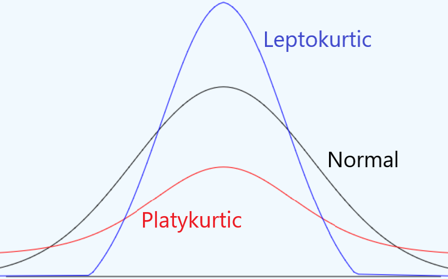 |
Example of different types of kurtosis. | Larry Green, CC-BY | CC-BY Michelle Oja |
| Leptokurtic | A tall and narrow distribution of data. | |
The tallest (blue) line is a leptokurtic shape. | Larry Green, CC-BY | CC-BY Michelle Oja |
| Platykurtic | A wide and flat distribution of data. | |
The lowest (red) line is a platykurtic shape. | Larry Green, CC-BY | CC-BY Michelle Oja |
| Mesokurtic | A medium, bell-sharped distribution of data. | |
The middle (black) line is a mesokurtic shape. | Larry Green, CC-BY | CC-BY Michelle Oja |
| Frequency Distribution | A distribution of data showing a count of frequency (how many) for each score or data point. | CC-BY Michelle Oja | |||
| Range | The difference between the highest score and the lowest score in a distribution of quantitative data. | CC-BY Michelle Oja | |||
| Robust | A term used by statisticians to mean resilient or resistant to | CC-BY-NC-SA Foster et al. | |||
| Descriptive Statistics | Used to describe or summarize the data from the sample. | CC-BY Michelle Oja | |||
| Inferential Statistics | Used to make generalizations from the sample data to the population of interest. | CC-BY Michelle Oja | |||
| Parameter | Statistic describing characteristics of the population (usually mean and standard deviation of the population) | CC-BY Michelle Oja | |||
| Non-Parametric Analysis, non-parametric analyses | Statistical analyses using ranked data; used when data sets are not normally distributed or with ranked data | CC-BY Michelle Oja | |||
| Research Hypothesis | A prediction of how groups are related. When comparing means, a complete research hypothesis includes:
|
CC-BY Michelle Oja | |||
| Null Hypothesis | A prediction that nothing is going on. The null hypothesis is always:
1. There is no difference between the groups’ means OR 2. There is no relationship between the variables. |
CC-BY Michelle Oja | |||
| Absolute value | Any number converted to a positive value | https://crumplab.github.io/statistic...ibingData.html | CC-BY-SA Mattew J. C. Crump | ||
| Main Effect | Any statistically significant differences between the levels of one independent variable in a factorial design. | CC-BY-SA Mattew J. C. Crump | |||
| Interaction, interaction effect | How the levels of two or more IVs jointly affect a DV; when one IV interacts with the other IV to affect the DV. | CC-BY Michelle Oja | |||
| Positive Correlation | When two quantitative variables vary together in the same direction; when one increases, the other one also increases (and when one decreases, the other also decreases) | CC-BY Michelle Oja | |||
| Negative Correlation | When two quantitative variables vary in opposite directions; when one variable increases, the other variable decreases. | CC-BY Michelle Oja | |||
| Binary variable, binary | A binary variable is a variable that only has two options (yes or no). Binary variables can be considered quantitative or qualitative. | CC-BY- Michelle Oja | |||
| Dichotomous variable, dichotomous | A dichotomous variable is a variable that only has two options (yes or no). Binary variables can be considered quantitative or qualitative. | CC-BY- Michelle Oja | |||