
8.1: Predicting a Population Mean
- Page ID
- 22078

\( \newcommand{\vecs}[1]{\overset { \scriptstyle \rightharpoonup} {\mathbf{#1}} } \)
\( \newcommand{\vecd}[1]{\overset{-\!-\!\rightharpoonup}{\vphantom{a}\smash {#1}}} \)
\( \newcommand{\dsum}{\displaystyle\sum\limits} \)
\( \newcommand{\dint}{\displaystyle\int\limits} \)
\( \newcommand{\dlim}{\displaystyle\lim\limits} \)
\( \newcommand{\id}{\mathrm{id}}\) \( \newcommand{\Span}{\mathrm{span}}\)
( \newcommand{\kernel}{\mathrm{null}\,}\) \( \newcommand{\range}{\mathrm{range}\,}\)
\( \newcommand{\RealPart}{\mathrm{Re}}\) \( \newcommand{\ImaginaryPart}{\mathrm{Im}}\)
\( \newcommand{\Argument}{\mathrm{Arg}}\) \( \newcommand{\norm}[1]{\| #1 \|}\)
\( \newcommand{\inner}[2]{\langle #1, #2 \rangle}\)
\( \newcommand{\Span}{\mathrm{span}}\)
\( \newcommand{\id}{\mathrm{id}}\)
\( \newcommand{\Span}{\mathrm{span}}\)
\( \newcommand{\kernel}{\mathrm{null}\,}\)
\( \newcommand{\range}{\mathrm{range}\,}\)
\( \newcommand{\RealPart}{\mathrm{Re}}\)
\( \newcommand{\ImaginaryPart}{\mathrm{Im}}\)
\( \newcommand{\Argument}{\mathrm{Arg}}\)
\( \newcommand{\norm}[1]{\| #1 \|}\)
\( \newcommand{\inner}[2]{\langle #1, #2 \rangle}\)
\( \newcommand{\Span}{\mathrm{span}}\) \( \newcommand{\AA}{\unicode[.8,0]{x212B}}\)
\( \newcommand{\vectorA}[1]{\vec{#1}} % arrow\)
\( \newcommand{\vectorAt}[1]{\vec{\text{#1}}} % arrow\)
\( \newcommand{\vectorB}[1]{\overset { \scriptstyle \rightharpoonup} {\mathbf{#1}} } \)
\( \newcommand{\vectorC}[1]{\textbf{#1}} \)
\( \newcommand{\vectorD}[1]{\overrightarrow{#1}} \)
\( \newcommand{\vectorDt}[1]{\overrightarrow{\text{#1}}} \)
\( \newcommand{\vectE}[1]{\overset{-\!-\!\rightharpoonup}{\vphantom{a}\smash{\mathbf {#1}}}} \)
\( \newcommand{\vecs}[1]{\overset { \scriptstyle \rightharpoonup} {\mathbf{#1}} } \)
\(\newcommand{\longvect}{\overrightarrow}\)
\( \newcommand{\vecd}[1]{\overset{-\!-\!\rightharpoonup}{\vphantom{a}\smash {#1}}} \)
\(\newcommand{\avec}{\mathbf a}\) \(\newcommand{\bvec}{\mathbf b}\) \(\newcommand{\cvec}{\mathbf c}\) \(\newcommand{\dvec}{\mathbf d}\) \(\newcommand{\dtil}{\widetilde{\mathbf d}}\) \(\newcommand{\evec}{\mathbf e}\) \(\newcommand{\fvec}{\mathbf f}\) \(\newcommand{\nvec}{\mathbf n}\) \(\newcommand{\pvec}{\mathbf p}\) \(\newcommand{\qvec}{\mathbf q}\) \(\newcommand{\svec}{\mathbf s}\) \(\newcommand{\tvec}{\mathbf t}\) \(\newcommand{\uvec}{\mathbf u}\) \(\newcommand{\vvec}{\mathbf v}\) \(\newcommand{\wvec}{\mathbf w}\) \(\newcommand{\xvec}{\mathbf x}\) \(\newcommand{\yvec}{\mathbf y}\) \(\newcommand{\zvec}{\mathbf z}\) \(\newcommand{\rvec}{\mathbf r}\) \(\newcommand{\mvec}{\mathbf m}\) \(\newcommand{\zerovec}{\mathbf 0}\) \(\newcommand{\onevec}{\mathbf 1}\) \(\newcommand{\real}{\mathbb R}\) \(\newcommand{\twovec}[2]{\left[\begin{array}{r}#1 \\ #2 \end{array}\right]}\) \(\newcommand{\ctwovec}[2]{\left[\begin{array}{c}#1 \\ #2 \end{array}\right]}\) \(\newcommand{\threevec}[3]{\left[\begin{array}{r}#1 \\ #2 \\ #3 \end{array}\right]}\) \(\newcommand{\cthreevec}[3]{\left[\begin{array}{c}#1 \\ #2 \\ #3 \end{array}\right]}\) \(\newcommand{\fourvec}[4]{\left[\begin{array}{r}#1 \\ #2 \\ #3 \\ #4 \end{array}\right]}\) \(\newcommand{\cfourvec}[4]{\left[\begin{array}{c}#1 \\ #2 \\ #3 \\ #4 \end{array}\right]}\) \(\newcommand{\fivevec}[5]{\left[\begin{array}{r}#1 \\ #2 \\ #3 \\ #4 \\ #5 \\ \end{array}\right]}\) \(\newcommand{\cfivevec}[5]{\left[\begin{array}{c}#1 \\ #2 \\ #3 \\ #4 \\ #5 \\ \end{array}\right]}\) \(\newcommand{\mattwo}[4]{\left[\begin{array}{rr}#1 \amp #2 \\ #3 \amp #4 \\ \end{array}\right]}\) \(\newcommand{\laspan}[1]{\text{Span}\{#1\}}\) \(\newcommand{\bcal}{\cal B}\) \(\newcommand{\ccal}{\cal C}\) \(\newcommand{\scal}{\cal S}\) \(\newcommand{\wcal}{\cal W}\) \(\newcommand{\ecal}{\cal E}\) \(\newcommand{\coords}[2]{\left\{#1\right\}_{#2}}\) \(\newcommand{\gray}[1]{\color{gray}{#1}}\) \(\newcommand{\lgray}[1]{\color{lightgray}{#1}}\) \(\newcommand{\rank}{\operatorname{rank}}\) \(\newcommand{\row}{\text{Row}}\) \(\newcommand{\col}{\text{Col}}\) \(\renewcommand{\row}{\text{Row}}\) \(\newcommand{\nul}{\text{Nul}}\) \(\newcommand{\var}{\text{Var}}\) \(\newcommand{\corr}{\text{corr}}\) \(\newcommand{\len}[1]{\left|#1\right|}\) \(\newcommand{\bbar}{\overline{\bvec}}\) \(\newcommand{\bhat}{\widehat{\bvec}}\) \(\newcommand{\bperp}{\bvec^\perp}\) \(\newcommand{\xhat}{\widehat{\xvec}}\) \(\newcommand{\vhat}{\widehat{\vvec}}\) \(\newcommand{\uhat}{\widehat{\uvec}}\) \(\newcommand{\what}{\widehat{\wvec}}\) \(\newcommand{\Sighat}{\widehat{\Sigma}}\) \(\newcommand{\lt}{<}\) \(\newcommand{\gt}{>}\) \(\newcommand{\amp}{&}\) \(\definecolor{fillinmathshade}{gray}{0.9}\)Let's get back to IQs.
IQ scores are defined to have mean 100 and standard deviation 15. How do we know that IQ scores have a true population mean of 100? Well, we know this because the people who designed the tests have administered them to very large samples, and have then “rigged” the scoring rules so that their sample has mean 100. That’s not a bad thing of course: it’s an important part of designing a psychological measurement. However, it’s important to keep in mind that this theoretical mean of 100 only attaches to the population that the test designers used to design the tests. Good test designers will actually go to some lengths to provide “test norms” that can apply to lots of different populations (for different age groups, for example).
This is very handy, but of course almost every research project of interest involves looking at a different population of people to those used in the test norms. For instance, suppose you wanted to measure the effect of low level lead poisoning on cognitive functioning in Port Pirie, a South Australian industrial town with a lead smelter. Perhaps you decide that you want to compare IQ scores among people in Port Pirie to a comparable sample in Whyalla, a South Australian industrial town with a steel refinery. Regardless of which town you’re thinking about, it doesn’t make a lot of sense simply to assume that the true population mean IQ is 100. No one has, to my knowledge, produced sensible norming data that can automatically be applied to South Australian industrial towns. We’re going to have to estimate the population parameters from a sample of data. So how do we do this?
Estimating the Population Mean
Suppose we go to Port Pirie and 100 of the locals are kind enough to sit through an IQ test. The average IQ score among these people turns out to be \(\bar{X} =98.5\). So what is the true mean IQ for the entire population of Port Pirie? Obviously, we don’t know the answer to that question. It could be 97.2, but if could also be 103.5. Our sampling isn’t exhaustive so we cannot give a definitive answer. Nevertheless if I was forced at gunpoint to give a “best guess” I’d have to say 98.5. That’s the essence of statistical estimation: giving a best guess.
In this example, estimating the unknown population parameter is straightforward. I calculate the sample mean, and I use that as my estimate of the population mean.
Estimating the Population Standard Deviation
What shall we use as our estimate in this case? Your first thought might be that we could do the same thing we did when estimating the mean, and just use the sample statistic as our estimate. That’s almost the right thing to do, but not quite.
Here’s why. Suppose I have a sample that contains a single observation. For this example, it helps to consider a sample where you have no intuitions at all about what the true population values might be, so let’s use something completely fictitious. Suppose the observation in question measures the cromulence of shoes. It turns out that my shoes have a cromulence of 20.
This is a perfectly legitimate sample, even if it does have a sample size of N=1. It has a sample mean of 20, and because every observation in this sample is equal to the sample mean (obviously!) it has a sample standard deviation of 0. As a description of the sample this seems quite right: the sample contains a single observation and therefore there is no variation observed within the sample. A sample standard deviation of s=0 is the right answer here. But as an estimate of the population standard deviation, it feels completely insane, right? Admittedly, you and I don’t know anything at all about what “cromulence” is, but we know something about data: the only reason that we don’t see any variability in the sample is that the sample is too small to display any variation! So, if you have a sample size of N=1, it feels like the right estimate of the population standard deviation is just to say “no idea at all”.
Notice that you don’t have the same intuition when it comes to the sample mean and the population mean. If forced to make a best guess about the population mean, it doesn’t feel completely insane to guess that the population mean is 20. Sure, you probably wouldn’t feel very confident in that guess, because you have only the one observation to work with, but it’s still the best guess you can make.
Let’s extend this example a little. Suppose I now make a second observation. The second set of shoes has a cromulence of 22. My data set now has N=2 observations of the cromulence of shoes. This time around, our sample is just large enough for us to be able to observe some variability: two observations is the bare minimum number needed for any variability to be observed! For our new data set, the sample mean is \(\bar{X} = 21\), and the sample standard deviation is s=1.
What intuitions do we have about the population? Again, as far as the population mean goes, the best guess we can possibly make is the sample mean: if forced to guess, we’d probably guess that the population mean cromulence is 21. What about the standard deviation? This is a little more complicated. The sample standard deviation is only based on two observations, and if you’re at all like me you probably have the intuition that, with only two observations, we haven’t given the population “enough of a chance” to reveal its true variability to us. It’s not just that we suspect that the estimate is wrong: after all, with only two observations we expect it to be wrong to some degree. The worry is that the error is systematic. Specifically, we suspect that the sample standard deviation is likely to be smaller than the population standard deviation.
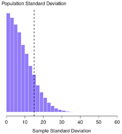
This intuition feels right, but it would be nice to demonstrate this somehow. There are in fact mathematical proofs that confirm this intuition, but unless you have the right mathematical background they don’t help very much. Instead, Dr. Navarro used statistical software to simulate the results of some experiments. With that in mind, let’s return to our IQ studies. Suppose the true population mean IQ is 100 and the standard deviation is 15. Dr. Navarro can generate the the results of an experiment in which N=2 IQ scores are measured, and calculate the sample standard deviation. If she does this over and over again, and plot a histogram of these sample standard deviations, what we have is the sampling distribution of the standard deviation (plotted in Figure \(\PageIndex{1}\)).
Samples Underestimate the Standard Deviation
The true population standard deviation is 15 (dashed line in Figure \(\PageIndex{1}\)), but as you can see from the histogram, the vast majority of experiments will produce a much smaller sample standard deviation than this. On average, this experiment would produce a sample standard deviation of only 8.5, well below the true value! In other words, the sample standard deviation is a biased estimate of the population standard deviation. In sum, even though the true population standard deviation is 15, the average of the sample standard deviations is only 8.5.
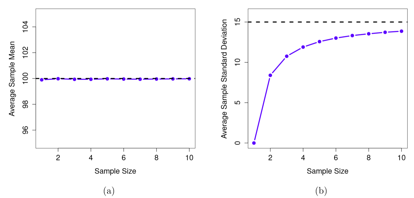
Now let’s extend the simulation. Instead of restricting ourselves to the situation where we have a sample size of N=2, let’s repeat the exercise for sample sizes from 1 to 10. If we plot the average sample mean and average sample standard deviation as a function of sample size, you get the results shown in Figure \(\PageIndex{2}\) Panel's (a) and (b). On the left hand side (panel a) is the plot of the average sample mean and on the right hand side (panel b) is the plot of the average standard deviation. The two plots are quite different. On average, the sample means turn out to be 100, regardless of sample size (panel a). However, the sample standard deviations turn out to be systematically too small (panel b), especially for small sample sizes. On average, the average sample mean is equal to the population mean. It is an unbiased estimator, which is essentially the reason why your best estimate for the population mean is the sample mean. The plot on the right is quite different: on average, the sample standard deviation s is smaller than the population standard deviation. It is a biased estimator. In other words, if we want to make a “best guess” about the value of the population standard deviation, we should make sure our guess is a little bit larger than the sample standard deviation.
How to Correctly Estimate the Population Standard Deviation from a Sample
The fix to this systematic bias turns out to be very simple. Here’s how it works. If you recall from Ch. 3 on Descriptive Statistics, the population's variance (the measure of variation before you square root into the standard deviation) is:
\[\sigma^{2}=\dfrac{\sum(X-\mu)^{2}}{N} \nonumber \]
As it turns out, we only need to make a tiny tweak to transform this into an unbiased estimator. All we have to do is divide by N−1 rather than by N. If we do that, we obtain the following formula:
\[s=\dfrac{\sum(X-\overline {X})^{2}}{N-1} \nonumber \]
This is an unbiased estimator of the population variance. A similar story applies for the standard deviation. If we divide by N−1 rather than N, our estimate of the population standard deviation becomes:
\[s=\sqrt{\dfrac{\sum(X-\overline {X})^{2}}{N-1}} \nonumber \]
One final point: in practice, a lot of people tend to refer to this estimated standard deviation of the population (i.e., the formula where we divide by \(N−1\)) as the sample standard deviation. Technically, this is incorrect: the sample standard deviation should be equal to s (i.e., the formula where we divide by N). These aren’t the same thing, either conceptually or numerically. One is a property of the sample, the other is an estimated characteristic of the population. However, in almost every real life application, what we actually care about is the estimate of the population parameter, and so people always report the standard deviation of the sample as the one with N-1 in the denominator. This is the right number to report, of course, it’s that people tend to get a little bit imprecise about terminology when they write it up, because “sample standard deviation” is shorter than “estimated population standard deviation”. It’s no big deal, and in practice I do the same thing everyone else does. Nevertheless, I think it’s important to keep the two concepts separate: it’s never a good idea to confuse “known properties of your sample” with “guesses about the population from which it came”.
Now that that is over, let's move into why we care about estimated the population's mean and standard deviation!