4.5: Normal Distributions and Probability Distributions

We will see shortly that the normal distribution is the key to how probability works for our purposes. To understand exactly how, let’s first look at a simple, intuitive example using pie charts.

Probability in Pie

Recall that a pie chart represents how frequently a category was observed and that all slices of the pie chart add up to 100%, or 1. This means that if we randomly select an observation from the data used to create the pie chart, the probability of it taking on a specific value is exactly equal to the size of that category’s slice in the pie chart.

Figure \(\PageIndex{1}\): Favorite Sports (CC-BY-NC-SA Foster et al. from An Introduction to Psychological Statistics)

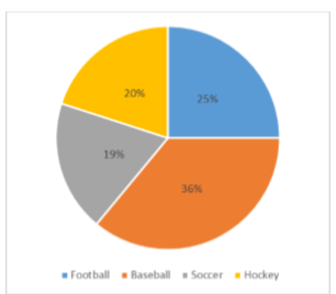
Take, for example, the pie chart in Figure \(\PageIndex{1}\) representing the favorite sports of 100 people. If you put this pie chart on a dart board and aimed blindly (assuming you are guaranteed to hit the board), the likelihood of hitting the slice for any given sport would be equal to the size of that slice. So, the probability of hitting the baseball slice is the highest at 36%. The probability is equal to the proportion of the chart taken up by that section.

We can also add slices together. For instance, maybe we want to know the probability to finding someone whose favorite sport is usually played on grass. The outcomes that satisfy this criteria are baseball, football, and soccer. To get the probability, we simply add their slices together to see what proportion of the area of the pie chart is in that region: \(36\% + 25\% + 20\% = 81\%\). We can also add sections together even if they do not touch. If we want to know the likelihood that someone’s favorite sport is not called football somewhere in the world (i.e. baseball and hockey), we can add those slices even though they aren’t adjacent or continuous in the chart itself: \(36\% + 20\% = 56\%\). We are able to do all of this because 1) the size of the slice corresponds to the area of the chart taken up by that slice, 2) the percentage for a specific category can be represented as a decimal (this step was skipped for ease of explanation above), and 3) the total area of the chart is equal to \(100\%\) or 1.0, which makes the size of the slices interpretable.

Normal Distributions

The normal distribution is the most important and most widely used distribution in statistics. It is sometimes called the “bell curve,” although the tonal qualities of such a bell would be less than pleasing. It is also called the “Gaussian curve” of Gaussian distribution after the mathematician Karl Friedrich Gauss.

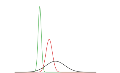
Strictly speaking, it is not correct to talk about “the normal distribution” since there are many normal distributions. Normal distributions can differ in their means and in their standard deviations. Figure \(\PageIndex{1}\) shows three normal distributions. The green (left-most) distribution has a mean of -3 and a standard deviation of 0.5, the distribution in red (the middle distribution) has a mean of 0 and a standard deviation of 1, and the distribution in black (right-most) has a mean of 2 and a standard deviation of 3. These as well as all other normal distributions are symmetric with relatively more values at the center of the distribution and relatively few in the tails. What is consistent about all normal distribution is the shape and the proportion of scores within a given distance along the x-axis. We will focus on the Standard Normal Distribution (also known as the Unit Normal Distribution), which has a mean of 0 and a standard deviation of 1 (i.e. the red distribution in Figure \(\PageIndex{1}\)).

Figure \(\PageIndex{1}\): Symmetrical Distributions with Different Means and Standard Deviations (CC-BY-NC-SA Foster et al. from An Introduction to Psychological Statistics)

Standard Normal Distribution

Important features of normal distributions are listed below.

1. Normal distributions are symmetric around their mean.
2. The mean, median, and mode of a normal distribution are equal. In Standard Normal Curves, the mean, median, and mode are all 0.
3. The area under the normal curve is equal to 1.0 (or 100% of all scores will fall somewhere in the distribution).
4. Normal distributions are denser in the center and less dense in the tails (bell-shaped).
5. There are known proportions of scores between the mean and each standard deviation.
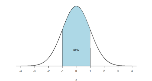
   1. One standard deviation- 68% of the area of a normal distribution is within one standard deviation of the mean (one standard deviation below the mean through one standard deviation above the mean).
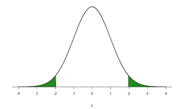
   2. Two standard deviations- Approximately 95% of the area of a normal distribution is within two standard deviations of the mean (two standard deviations below the mean through two standard deviations above the mean).

These properties enable us to use the normal distribution to understand how scores relate to one another within and across a distribution.

Probability in Normal Distributions

Play with this applet to learn about probability distributions (website address: http://www.rossmanchance.com/applets/OneProp/OneProp.htm?candy=1)

Probability distributions are what make statistical analyses work. Each distribution of events from any sample can be “translated” into a probability distribution, then used to predict the probability of that event happening!

Just like a pie chart is broken up into slices by drawing lines through it, we can also draw a line through the normal distribution to split it into sections. We know that one standard deviation below the mean to one standard deviation above the mean contains 68% of the area under the curve because we know the properties of standard normal curves.

Figure \(\PageIndex{2}\): There is a 68% chance of selection a Score from the shaded region (CC-BY-NC-SA Foster et al. from An Introduction to Psychological Statistics)

This time, let’s find the area corresponding to the extreme tails. For standard normal curves, 95% of scores should be in the middle section of Figure \(\PageIndex{3}\), and a total of 5% in the shaded areas. Since there are two shaded areas, that's about 2.5% on each side.

Figure \(\PageIndex{3}\): Area Beyond 2 Standard Deviations (CC-BY-NC-SA Foster et al. from An Introduction to Psychological Statistics)

Those important characteristics of a Standard Normal Distribution are deceptively simple, so let's put some of these ideas together to see what we get.

Law of Large Numbers: I know through the Law of Large Numbers that if I have enough data, then my sample will begin to become more and more "normal' (have the characteristics of a normally distributed population, including the important characteristics above).

Probability Distributions: I know that I can make predictions from probability distributions. I can use probability distributions to understand the likelihood of specific events happening.

Standard Normal Curve: I know that there should be specific and predictable proportions (percentages) of scores between the mean and each standard deviation away from the mean.

Together, these features will allow you to:

• Predict the probability of events happening.
• Estimate how many people might be affected based on sample size.
• Test Research Hypotheses about different groups.

This is the magic of the Standard Normal Curve!

Non-Parametric Distributions

One last thing...

There's a lot of heavy lifting for the Standard Normal Distribution. But what if your sample, or even worse, the population, is not normally distributed? That's when non-parametric statistics come in.

A parameter is a statistic that describes the population. Non-parametric statistics don’t require the population data to be normally distributed. Most of the analyses that we'll conduct compare means (a measure of central tendency) of different groups. But if the data are not normally distributed, then we can’t compare means because there is no center! Non-normal distributions may occur when there are:

• Few people (small N)
• Extreme scores (outliers)
• There’s an arbitrary cut-off point on the scale. (Like if a survey asked for ages, but then just said, “17 and below”.)

The reason that I bring this up is because sometimes you just can't run the statistics that we're going to learn about because the population's data is not normally distributed. Since the Standard Normal Curve is the basis for most types of statistical inferences, you can't use these (parametric) analyses with data that they don't fit. We'll talk about alternative analyses for some of the common (parametric) statistical analyses, but you heard it here first! Non-parametric distributions are when the population is not normally distributed.

Okay, onward to learning more about how the Standard Normal Curve is important...