
Lab 8: More ANOVA
- Page ID
- 9049
\( \newcommand{\vecs}[1]{\overset { \scriptstyle \rightharpoonup} {\mathbf{#1}} } \)
\( \newcommand{\vecd}[1]{\overset{-\!-\!\rightharpoonup}{\vphantom{a}\smash {#1}}} \)
\( \newcommand{\dsum}{\displaystyle\sum\limits} \)
\( \newcommand{\dint}{\displaystyle\int\limits} \)
\( \newcommand{\dlim}{\displaystyle\lim\limits} \)
\( \newcommand{\id}{\mathrm{id}}\) \( \newcommand{\Span}{\mathrm{span}}\)
( \newcommand{\kernel}{\mathrm{null}\,}\) \( \newcommand{\range}{\mathrm{range}\,}\)
\( \newcommand{\RealPart}{\mathrm{Re}}\) \( \newcommand{\ImaginaryPart}{\mathrm{Im}}\)
\( \newcommand{\Argument}{\mathrm{Arg}}\) \( \newcommand{\norm}[1]{\| #1 \|}\)
\( \newcommand{\inner}[2]{\langle #1, #2 \rangle}\)
\( \newcommand{\Span}{\mathrm{span}}\)
\( \newcommand{\id}{\mathrm{id}}\)
\( \newcommand{\Span}{\mathrm{span}}\)
\( \newcommand{\kernel}{\mathrm{null}\,}\)
\( \newcommand{\range}{\mathrm{range}\,}\)
\( \newcommand{\RealPart}{\mathrm{Re}}\)
\( \newcommand{\ImaginaryPart}{\mathrm{Im}}\)
\( \newcommand{\Argument}{\mathrm{Arg}}\)
\( \newcommand{\norm}[1]{\| #1 \|}\)
\( \newcommand{\inner}[2]{\langle #1, #2 \rangle}\)
\( \newcommand{\Span}{\mathrm{span}}\) \( \newcommand{\AA}{\unicode[.8,0]{x212B}}\)
\( \newcommand{\vectorA}[1]{\vec{#1}} % arrow\)
\( \newcommand{\vectorAt}[1]{\vec{\text{#1}}} % arrow\)
\( \newcommand{\vectorB}[1]{\overset { \scriptstyle \rightharpoonup} {\mathbf{#1}} } \)
\( \newcommand{\vectorC}[1]{\textbf{#1}} \)
\( \newcommand{\vectorD}[1]{\overrightarrow{#1}} \)
\( \newcommand{\vectorDt}[1]{\overrightarrow{\text{#1}}} \)
\( \newcommand{\vectE}[1]{\overset{-\!-\!\rightharpoonup}{\vphantom{a}\smash{\mathbf {#1}}}} \)
\( \newcommand{\vecs}[1]{\overset { \scriptstyle \rightharpoonup} {\mathbf{#1}} } \)
\(\newcommand{\longvect}{\overrightarrow}\)
\( \newcommand{\vecd}[1]{\overset{-\!-\!\rightharpoonup}{\vphantom{a}\smash {#1}}} \)
\(\newcommand{\avec}{\mathbf a}\) \(\newcommand{\bvec}{\mathbf b}\) \(\newcommand{\cvec}{\mathbf c}\) \(\newcommand{\dvec}{\mathbf d}\) \(\newcommand{\dtil}{\widetilde{\mathbf d}}\) \(\newcommand{\evec}{\mathbf e}\) \(\newcommand{\fvec}{\mathbf f}\) \(\newcommand{\nvec}{\mathbf n}\) \(\newcommand{\pvec}{\mathbf p}\) \(\newcommand{\qvec}{\mathbf q}\) \(\newcommand{\svec}{\mathbf s}\) \(\newcommand{\tvec}{\mathbf t}\) \(\newcommand{\uvec}{\mathbf u}\) \(\newcommand{\vvec}{\mathbf v}\) \(\newcommand{\wvec}{\mathbf w}\) \(\newcommand{\xvec}{\mathbf x}\) \(\newcommand{\yvec}{\mathbf y}\) \(\newcommand{\zvec}{\mathbf z}\) \(\newcommand{\rvec}{\mathbf r}\) \(\newcommand{\mvec}{\mathbf m}\) \(\newcommand{\zerovec}{\mathbf 0}\) \(\newcommand{\onevec}{\mathbf 1}\) \(\newcommand{\real}{\mathbb R}\) \(\newcommand{\twovec}[2]{\left[\begin{array}{r}#1 \\ #2 \end{array}\right]}\) \(\newcommand{\ctwovec}[2]{\left[\begin{array}{c}#1 \\ #2 \end{array}\right]}\) \(\newcommand{\threevec}[3]{\left[\begin{array}{r}#1 \\ #2 \\ #3 \end{array}\right]}\) \(\newcommand{\cthreevec}[3]{\left[\begin{array}{c}#1 \\ #2 \\ #3 \end{array}\right]}\) \(\newcommand{\fourvec}[4]{\left[\begin{array}{r}#1 \\ #2 \\ #3 \\ #4 \end{array}\right]}\) \(\newcommand{\cfourvec}[4]{\left[\begin{array}{c}#1 \\ #2 \\ #3 \\ #4 \end{array}\right]}\) \(\newcommand{\fivevec}[5]{\left[\begin{array}{r}#1 \\ #2 \\ #3 \\ #4 \\ #5 \\ \end{array}\right]}\) \(\newcommand{\cfivevec}[5]{\left[\begin{array}{c}#1 \\ #2 \\ #3 \\ #4 \\ #5 \\ \end{array}\right]}\) \(\newcommand{\mattwo}[4]{\left[\begin{array}{rr}#1 \amp #2 \\ #3 \amp #4 \\ \end{array}\right]}\) \(\newcommand{\laspan}[1]{\text{Span}\{#1\}}\) \(\newcommand{\bcal}{\cal B}\) \(\newcommand{\ccal}{\cal C}\) \(\newcommand{\scal}{\cal S}\) \(\newcommand{\wcal}{\cal W}\) \(\newcommand{\ecal}{\cal E}\) \(\newcommand{\coords}[2]{\left\{#1\right\}_{#2}}\) \(\newcommand{\gray}[1]{\color{gray}{#1}}\) \(\newcommand{\lgray}[1]{\color{lightgray}{#1}}\) \(\newcommand{\rank}{\operatorname{rank}}\) \(\newcommand{\row}{\text{Row}}\) \(\newcommand{\col}{\text{Col}}\) \(\renewcommand{\row}{\text{Row}}\) \(\newcommand{\nul}{\text{Nul}}\) \(\newcommand{\var}{\text{Var}}\) \(\newcommand{\corr}{\text{corr}}\) \(\newcommand{\len}[1]{\left|#1\right|}\) \(\newcommand{\bbar}{\overline{\bvec}}\) \(\newcommand{\bhat}{\widehat{\bvec}}\) \(\newcommand{\bperp}{\bvec^\perp}\) \(\newcommand{\xhat}{\widehat{\xvec}}\) \(\newcommand{\vhat}{\widehat{\vvec}}\) \(\newcommand{\uhat}{\widehat{\uvec}}\) \(\newcommand{\what}{\widehat{\wvec}}\) \(\newcommand{\Sighat}{\widehat{\Sigma}}\) \(\newcommand{\lt}{<}\) \(\newcommand{\gt}{>}\) \(\newcommand{\amp}{&}\) \(\definecolor{fillinmathshade}{gray}{0.9}\)Objective:
1. Understand when and how to perform post hoc analysis of a significant ANOVA \(F\) test for comparing three or more population means.
2. Understand how to perform ANOVA using a permutation test.
Definitions:
- pairwise comparisons
- post hoc test
- Tukey's HSD method
- classes (produced by post hoc analysis of ANOVA results)
Introduction:
In Lab 7, we considered a technique for testing claims about three or more population means known as analysis of variance (ANOVA). In particular, we used the classical approach to performing ANOVA based on the \(F\) distribution. The classical approach requires that the populations being compared are normally distributed with equal variances. In this lab, we will see how to use the permutation test procedure, introduced in Lab 2, to perform ANOVA when these requirements do not appear to be met.
Before developing the permutation test for ANOVA, we will discuss what to do after obtaining a significant result for the ANOVA \(F\) test.
Activities:
Getting Organized: If you are already organized, and remember the basic protocol from previous labs, you can skip this section.
Navigate to your class folder structure. Within your "Labs" folder make a subfolder called "Lab8". Next, download the lab notebook .Rmd file for this lab from Blackboard and save it in your "Lab8" folder. You will again be working with the Zombies.csv data set on this lab. You should either re-download the data file into your "Lab8" folder from Blackboard, or just copy the file from your "Lab7" folder into the "Lab8" folder.
Within RStudio, navigate to your "Lab8" folder via the file browser in the lower right pane and then click "More > Set as working directory". Get set to write your observations and R commands in an R Markdown file by opening the "lab8_notebook.Rmd" file in RStudio. Remember to add your name as the author in line 3 of the document. For this lab, enter all of your commands into code chunks in the lab notebook. You can still experiment with code in an R script, if you want. To set up an R Script in RStudio, in the upper left corner click “File > New File > R script”. A new tab should open up in the upper left pane of RStudio.
After ANOVA: If an ANOVA test is significant, then all we know is that there is a difference, but we don't know exactly what the difference is. For example, let's revisit the four chemical plants we considered in Lab 7. Recall that we analyzed the amount of polluting effluents per gallon in samples of liquid waste discharged from the four plants. We used the following code to perform an ANOVA \(F\) test to determine if there is a significant difference between the mean weight of polluting effluents discharged by the four plants (note that the data below are slightly different than the data used in Lab 7):
Waste = c(1.65, 1.72, 1.50, 1.37, 1.60,
          1.70, 1.85, 1.56, 2.05,
          1.40, 1.75, 1.38, 1.65, 1.55,
          2.10, 1.95, 1.75, 1.88)
Plant = rep(c("A", "B", "C", "D"), c(5, 4, 5, 4))
aov.pollution = aov(Waste ~ Plant)
summary(aov.pollution)

##                Df  Sum Sq  Mean Sq   F value  Pr(>F)
## Plant           3  0.4297  0.14323      5.39  0.0112 *
## Residuals      14  0.3720  0.02657
## ---
## Signif. codes:  0 '***' 0.001 '**' 0.01 '*' 0.05 '.' 0.1 ' ' 1
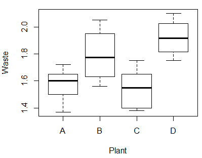
From the ANOVA table, we see that the \(P\)-value is significant at the \(\alpha=0.05\) level, so we conclude that there is sufficient evidence that the mean weight of polluting effluents discharged by the four plants is not equal. However, this result alone says nothing about which plant or plants have the largest mean or the smallest.
If we look at side-by-side boxplots of the sample waste amounts across the four plants, we can see that the sample from plant D appears to have the highest mean and plant C the lowest. But is the mean for plant D significantly higher than the mean for plant B? In other words, when we make pairwise comparisons between the plant means are the differences significant? To answer this question, we need to run more hypothesis tests.
_____________________________________________________
Pause for Reflection #1:
Why do we need to run more hypothesis tests to determine whether the differences in the means between the pairs are significant? Why isn't it enough to just look at the side-by-side boxplots?
_____________________________________________________
Post Hoc Tests: As we discussed in class, we cannot simply perform a series of independent samples \(t\) tests for each pairwise comparison because it is not efficient and it inflates the possibility of committing a Type I error. Instead, we will perform a post hoc test. Generally speaking, a post hoc test is a test of significance that decreases the probability of making a Type I error. In particular, we will look at using the post hoc test given by Tukey's HSD (honestly significant difference).
The method of Tukey's HSD is to simultaneously construct confidence intervals for all differences \((\mu_i-\mu_j\)) that collectively hold at the desired confidence level. The pairwise comparisons are then made as follows:
- If the confidence interval for (\(\mu_i - \mu_j\)) includes 0, then \(\mu_i\) and \(\mu_j\) are not significantly different.
- If the confidence interval for (\(\mu_i - \mu_j\)) does not include 0, then \(\mu_i\) and \(\mu_j\) are significantly different.
Tukey's method is performed in R by calling the function TukeyHSD() on the results of the ANOVA \(F\) test. For the pollution example, try the following:
TukeyHSD(aov.pollution, conf.level = 0.95) # default conf.level is 95%
In the table produced by the above code, the diff column gives the difference in the observed sample means, lwr gives the lower end point of the confidence interval, upr gives the upper end point and p adj gives the p-value after adjustment for the multiple comparisons. Note that we can also visualize the results of Tukey's method by calling the plot() function on the results:
plot(TukeyHSD(aov.pollution))
_____________________________________________________
Pause for Reflection #2:
Using the results of Tukey's method, identify which pairs of chemical plants appear to have significantly different means. Then sort the plants into classes, where each class contains plants that have similar means (i.e., means that were determined to not be significantly different). It may be helpful to redo the side-by-side boxplot so that the plots are placed in order of decreasing means (the default ordering is alphabetical):
Plant = factor(Plant, levels = c("D", "B", "A", "C")) # reorder the labels
boxplot(Waste ~ Plant)
_____________________________________________________
Permutation Test for ANOVA: In Lab 7 and in class on Tuesday, we explored using simulation to see what happens when the assumptions required for the ANOVA \(F\) test are not met. Specifically, we saw that when the data do not support the assumption of equal variance for the populations, the risk of making a Type I error increases.
For example, let's revisit the data set in the Zombies.csv file, containing data about the number of zombies killed (killed) and by what household weapon (weapon) for a sample of 31 apocalypse survivors. Using the tapply() function, we can compute the variances for the samples across the weapons:
Zombies = read.csv("Zombies.csv")
tapply(Zombies$killed, Zombies$weapon, var)

## baseball bat        chainsaw        golf club
##     6.454545        6.011111         2.322222
Based on these results, we may question the validity of assuming that the population variances are equal, which then calls into question the reliability of an ANOVA performed using the \(F\) test approach.
In the case that the assumptions of the \(F\) test do not appear to be met, we can use the ideas presented in Lab 2 to form a permutation distribution of the test statistic, rather than using the \(F\) distribution. Specifically, the permutation test approach for performing ANOVA uses the following steps:
1. randomly permute the group labels on the observations;
2. compute the test statistic given by the ratio of the between group variability to the within group variability (i.e., MSTR/MSE) for the new groups using the permuted labels;
3. repeat steps 1 & 2 many times storing the resulting test statistic;
4. compute the \(P\)-value by finding the proportion of times the resulting test statistics from steps 1 & 2 exceed the original observed test statistic.
The following code implements the permutation test approach to ANOVA for the Zombie example:
observed = summary(aov(Zombies$killed ~ Zombies$weapon))[[1]][1,4]     #original observed test statistic

n = length(Zombies$killed)                                             #total number of observations
N = 10^4 - 1                                                           #number of times to repeat permutation of labels
results = numeric(N)

for (i in 1:N)
{
  index = sample(n)                                                    #create permutation of numbers 1 to n
  killed.perm = Zombies$killed[index]                                  #reorder observations in killed using permutation
  results[i] = summary(aov(killed.perm ~ Zombies$weapon))[[1]][1,4]    #store new value of test statistic
}

(sum(results >= observed) + 1) / (N + 1)                          #P-value
_____________________________________________________
Pause for Reflection #3:
Run the above code to perform the permutation test. Record the \(P\)-value you find in your lab notebook and compare the results to what you found in Lab 7 when performing the ANOVA \(F\) test. Comment on whether you think that a permutation test was necessary.
_____________________________________________________
Pause for Reflection #4:
Comment on why the \(P\)-value of the permutation test for ANOVA is given by the proportion of times the resulting test statistics for the permutations exceed the original observed test statistic. In particular, explain why a test statistic for a permutation that is as large or larger than what was originally observed is considered more extreme in this context.
_____________________________________________________