Lab 5: Confidence Intervals

Objectives:

1. Find confidence intervals for \(\mu\).
2. Explore the \(t\) distribution.

Definitions:

• point estimate vs. interval estimate
• confidence intervals
• confidence level
• t distribution

Introduction:

In the past few weeks, we have learned how to find point estimates for population parameters, in other words, single value estimates of an unknown parameter. But these point estimates are based on random samples and so are inherently variable and uncertain. We can model that uncertainty with the sampling distribution of a statistic, and last week we focused on the sampling distribution of the sample mean. This week, we use that sampling distribution to construct interval estimates for population parameters. Interval estimates give a range of plausible values for a parameter based on a random sample, and incorporate the variability of point estimates.

Activities:

Getting Organized: If you are already organized, and remember the basic protocol from previous labs, you can skip this section.

Navigate to your class folder structure. Within your "Labs" folder make a subfolder called "Lab5". Next, download the lab notebook .Rmd file for this lab from Blackboard and save it in your "Lab5" folder. You will be working with the NCBirths2004 dataset on this lab. You should download the data file into your "Lab5" folder from Blackboard.

Within RStudio, navigate to your "Lab5" folder via the file browser in the lower right pane and then click "More > Set as working directory". Get set to write your observations and R commands in an R Markdown file by opening the "lab5_notebook.Rmd" file in RStudio. Remember to add your name as the author in line 3 of the document. For this lab, enter all of your commands into code chunks in the lab notebook. You can still experiment with code in an R script, if you want. To set up an R Script in RStudio, in the upper left corner click “File > New File > R script”. A new tab should open up in the upper left pane of RStudio.

 

Confidence Intervals for a Mean, Variance Known: At the end of class on Tuesday, we looked at estimating the mean birth weight for girls born in South Bend. We assumed that the population of birth weights was normally distributed with unknown mean \(\mu\), but known standard deviation \(\sigma = 1.1\). In that case, the sampling distribution of a sample mean birth weight for a random sample of size \(n=100\) is normal with mean \(\mu\) and standard deviation \(1.1/\sqrt{100}\). Given this, we then derived the following:

\(\displaystyle{0.95 = P(-1.96 < Z < 1.96) = P\left(-1.96 < \frac{\bar{X} - \mu}{1.1/\sqrt{100}} < 1.96\right) = P\left(\bar{X}-1.96 \frac{1.1}{\sqrt{100}} < \mu < \bar{X}+1.96 \frac{1.1}{\sqrt{100}}\right)}\)

The random interval given by

\(\displaystyle{\left(\bar{X} - 1.96\frac{1.1}{\sqrt{100}},\ \bar{X} + 1.96\frac{1.1}{\sqrt{100}}\right)}\)    (1)

has a probability of 0.95 of containing the true value of the mean \(\mu\). Now, once the public health officials in South Bend have drawn a random sample, the random variable \(\bar{X}\) is replaced by the (observed) sample mean birth weight of \(\bar{x} = 7.1\) lb, giving the specific interval

\(\displaystyle{\left(7.1 - 1.96\frac{1.1}{\sqrt{100}},\ 7.1 + 1.96\frac{1.1}{\sqrt{100}}\right) \quad\Rightarrow\quad (6.884, 7.316)},\)    (2)

which is no longer random. We interpret this interval by saying that we are 95% confident that the population mean birth weight of girls born in South Bend is between 6.9 and 7.3 lb. In other words, if we repeated the same process of drawing samples and computing intervals many times, then in the long run, 95% of the intervals would include \(\mu\).

_____________________________________________________

Pause for Reflection #1:

Explain in your own words why the interval in equation (1) is random, but the interval in equation (2) is not.

_____________________________________________________

 

In general, if a random sample of size \(n\) is drawn from a normal distribution with unknown mean \(\mu\) and known standard deviation \(\sigma\), then a 95% confidence interval for \(\mu\) is

\(\displaystyle{\left(\bar{X} - 1.96\frac{\sigma}{\sqrt{n}},\ \bar{X} + 1.96\displaystyle \frac{\sigma}{\sqrt{n}}\right)}\)     (3)

If we repeatedly draw random samples from the population and compute the above 95% confidence interval for each sample, then we expect about 95 of those intervals will contain the actual value of \(\mu\).

We can demonstrate the interpretation of confidence intervals with a simulation. The following code simulates drawing random samples of size 30 from a \(N(25, 4)\) distribution. For each sample, we construct the 95% confidence interval and check to see if it contains the population mean, \(\mu = 25\). We do this 1000 times and keep track of the number of times the interval contains \(\mu\) using a counter. We can also visualize the first 100 intervals computed.
 

counter = 0                                       # set counter to 0
plot(x = c(22, 28), y = c(1, 100), type = "n",    # set up a blank plot
     xlab = "", ylab = "")                        # with no axis labels
for (i in 1:1000)
{
  x = rnorm(30, 25, 4)                            # draw random sample of size 30
  L = mean(x) - 1.96*4/sqrt(30)                   # lower endpoint of interval
  U = mean(x) + 1.96*4/sqrt(30)                   # upper endpoint of interval
  if (L < 25 && 25 < U)                           # check if 25 is in interval
    counter = counter + 1                         # if yes, increase counter by 1
  if (i <= 100)                                   # plot first 100 intervals
    segments(L, i, U, i)
}
abline(v = 25, col = "red")                       # vertical line at mu
counter/1000                                      # proportion of times mu in interval

 

_____________________________________________________

Pause for Reflection #2:

In your lab notebook, run the above simulation (code provided) and comment on the proportion of times the intervals in the simulation contain \(\mu = 25\). Is it close to 95%?

Explain in your own words what the plot produced by the simulation demonstrates.

_____________________________________________________

 

In the first example with birth weights and the above simulation, we constructed 95% confidence intervals. The formula in equation (3) was derived starting from the fact that for the standard normal random variable \(Z\), we have

\(0.95 = P(-1.96 < Z < 1.96).\)

This fact can be confirmed using the qnorm() function in R, which calculates quantiles for the normal distribution given a probability. With 0.95 probability in the middle, that leaves 0.05/2 = 0.025 probability in each of the two tails, as Figure 1 demonstrates.

 

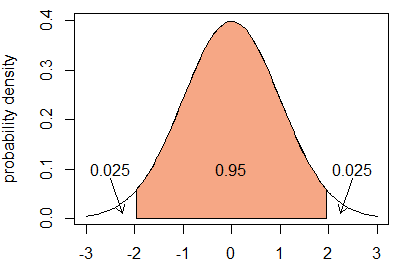
Figure 1: Standard normal density with shaded area 0.95

In this case, we also have that \(0.025 = P(Z > 1.96)\), which is found in R as follows:

qnorm(0.025, lower.tail = FALSE)      # returns the value q such that P(Z > q) = 0.025

 

_____________________________________________________

Pause for Reflection #3:

If we want 0.93 probability in the middle of a standard normal density curve, how much probability does that leave in each of the two tail regions? Sketch a figure similar to Figure 1, but with 0.93 middle probability and upload the image to your lab notebook. Use the qnorm() function to find the value of \(q\) satisfying \(0.93 = P(-q < Z < q)\).

 

_____________________________________________________

Pause for Reflection #4:

Redo the simulation above, but find 93% confidence intervals this time. You will need to use the value of \(q\) you found in Reflection #3 and alter in some way the following two lines in the for loop of the simulation:

  L = mean(x) - 1.96*4/sqrt(30)                   # lower endpoint of interval
  U = mean(x) + 1.96*4/sqrt(30)                   # upper endpoint of interval

What is the proportion of times the intervals in the simulation contain \(\mu = 25\) equal to now? Is it what you expected? Explain.

_____________________________________________________

 

In general, we let \(z_{\alpha/2}\) denote the \((1-\alpha/2)\) quantile for the standard normal distribution. In other words, \(z_{\alpha/2}\) is the value such that \(P(Z > z_{\alpha/2}) = \alpha/2\). By symmetry then, the middle probability given by \((1-\alpha)\) falls between \(-z_{\alpha/2}\) and \(z_{\alpha/2}\). (See Figure 2 below.) For example, in a 95% confidence interval, \(\alpha = 0.05\) and \(z_{\alpha/2} = z_{0.025} = 1.96\).

 

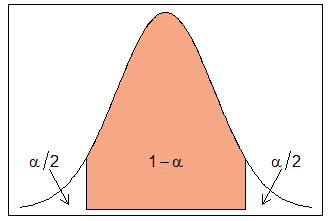
Figure 2: Standard normal density with shaded area (1-alpha)

 

We can now give a general formula for a \(100(1-\alpha)\)% confidence interval of \(\mu\), when \(\sigma\) is know.

 

Z Confidence Interval for a Normal Mean with Known Standard Deviation

If \(X_i\sim N(\mu, \sigma)\), for \(i=1,\ldots,n\), with \(\sigma\) known, then a \(100(1-\alpha)\)% confidence interval for \(\mu\) is given by

\(\displaystyle{\left(\bar{X} - z_{\alpha/2} \frac{\sigma}{\sqrt{n}},\ \bar{X} + z_{\alpha/2} \frac{\sigma}{\sqrt{n}}\right)}\)

 

_____________________________________________________

Pause for Reflection #5:

Return to the first example and find a 90% confidence interval for the mean birth weight of girls born in South Bend. How does this interval compare to the 95% confidence interval we found? Which interval is wider?

_____________________________________________________

 

Confidence Intervals for a Mean, Variance Unknown: In practice, we will not know either the mean or the standard deviation of the population we are interested in. As we have seen in previous weeks, if we want to know the value of a population parameter, we can use a statistic computed from a random sample to estimate it. As we use \(\bar{X}\) to estimate \(\mu\), we can use \(S\), the sample standard deviation, to estimate \(\sigma\). This leads to the question: does replacing \(\sigma\) with \(S\) in the following change the distribution?

\(\displaystyle{Z = \frac{\bar{X} - \mu}{\sigma/\sqrt{n}} \sim N(0,1) \quad\Rightarrow\quad T = \frac{\bar{X} - \mu}{\textcolor{red}{S}/\sqrt{n}} \stackrel{?}{\sim} N(0,1)}\)

It turns out that estimating \(\sigma\) with \(S\) does indeed change the sampling distribution. As we have done many times already, we explore this question with a simulation.

N = 10^4
z = numeric(N)
t = numeric(N)
n = 15                                # sample size
for (i in 1:N)
{
  x = rnorm(n, 25, 4)                 # draw 15 numbers from N(25, 4)
  Xbar = mean(x)                      # calculate sample mean
  S = sd(x)                           # calculate sample sd
  z[i] = (Xbar - 25) / (4/sqrt(n))    # standardize sample mean using sigma
  t[i] = (Xbar - 25) / (S/sqrt(n))    # standardize sample mean using sample sd
}
hist(z)
hist(t)
qqnorm(z); qqline(z)                  # assess normality for z
qqnorm(t); qqline(t)                  # assess normality for 

_____________________________________________________

Pause for Reflection #6:

In your lab notebook, run the above simulation (code provided). Explain how the results of the simulation show that the distribution of \(T = (\bar{X} - \mu)/(S/\sqrt{n})\) is not normally distributed.

_____________________________________________________

 

The distribution of \(T = (\bar{X} - \mu)/(S/\sqrt{n})\) is actually a Student's t distribution with \(n-1\) degrees of freedom, provided that the population is normally distributed. The pdf of \(t\) distribution with \(k\) degrees of freedom is bell-shaped and symmetric about 0, like the standard normal pdf. But, unlike the standard normal pdf, it has thicker tails. As \(k\) tends to infinity, the pdf of the \(t\) distribution approaches the standard normal pdf. Figure 3 below shows the pdf's for the standard normal distribution and three \(t\) distributions.

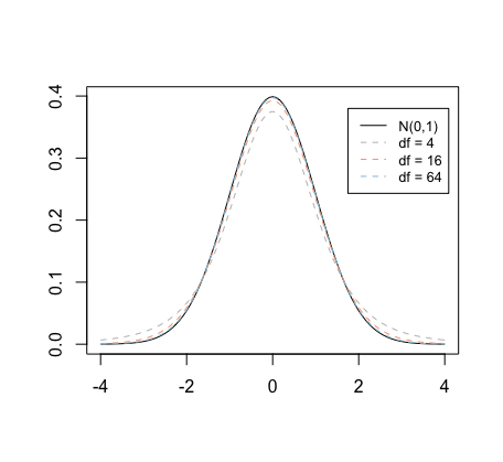
Figure 3: Comparison of pdf's for standard normal and t distributions

We derive the confidence interval for \(\mu\) when \(\sigma\) is unknown in the same way as when \(\sigma\) is know, except we use the \(t\) distribution to find quantiles. We let \(t_{\alpha/2, n-1}\) denote the \((1-\alpha)\) quantile for a \(t\) distribution with \(n-1\) degrees of freedom, i.e., the value such that

\(P(T > t_{\alpha/2, n-1}) = \alpha/2,\)

where \(T\) has a \(t\) distribution with \(n-1\) degrees of freedom. The quantiles \(t_{\alpha/2, n-1}\) replace the standard normal quantiles \(z_{\alpha/2}\) in the formula, and we arrive at the following.

 

T Confidence Interval for a Normal Mean with Unknown Standard Deviation

If \(X_i\sim N(\mu, \sigma)\), for \(i=1,\ldots,n\), with \(\sigma\) known, then a \(100(1-\alpha)%\) confidence interval for \(\mu\) is given by

\(\displaystyle{\left(\bar{X} - t_{\alpha/2, n-1}\frac{S}{\sqrt{n}},\ \bar{X} + t_{\alpha/2, n-1} \frac{S}{\sqrt{n}}\right)}\)

 

The functions pt() and qt() give probabilities and quantiles, respectively, for the \(t\) distribution. For example, to find \(P(T < 2.8)\) for the random variable \(T\) from a \(t\) distribution with 27 degrees of freedom, try the following:

pt(2.8, 27)

And to find the quantile \(t_{0.05, 27}\), try

qt(0.05, 27, lower.tail = FALSE)

_____________________________________________________

Pause for Reflection #7:

Compare the quantile \(t_{0.05, 27}\) to the corresponding standard normal quantile \(z_{0.05}\). Which one is larger? Can you explain why? What effect on the width of a 90% confidence interval does using the \(t\) distribution quantile have? Can you explain why this makes sense given that confidence intervals based on the \(t\) distribution are used when \(\sigma\) is unknown?

 

_____________________________________________________

Pause for Reflection #8:

Suppose that the public health officials in South Bend are also interested the mean birth weight of boys in their city. They are willing to again suppose that the distribution of boys weights in South Bend is normal, but they do not want to assume a value for the standard deviation. Instead, they obtain a random sample of 28 boys, resulting a sample mean of 7.6 lb and a sample standard deviation of 1.3 lb. Use their results to construct a 90% confidence interval for the true mean birth weight of boys born in South Bend. Upload an image of any hand-written work.

_____________________________________________________

 

If you have the full data set of observations in a random sample available in R, then the function t.test() can calculate confidence intervals quickly. We will demonstrate this with the NCBirths2004 data set, which contains information on a random sample of 1009 babies born in North Carolina during 2004, and construct a 99% confidence interval for the mean birth weight (in grams) of girls born in North Carolina.
 

NCBirths2004 = read.csv("NCBirths2004.csv")
girls = subset(NCBirths2004, select = Weight, subset = Gender == "Female", drop = TRUE)
t.test(girls, conf.level = 0.99)$conf

## [1] 3343.305 3453.328
## attr(,"conf.level")
## [1] 0.99

 

Thus, the 99% confidence interval for the mean birth weight of girls born in North Carolina in 2004 is (3343.3, 3453.3) g.

_____________________________________________________

Pause for Reflection #9:

Alter the t.test() function and find 95% and 90% confidence intervals for the mean birth weight of girls born in North Carolina in 2004. How do these intervals compare to each other and to the 99% confidence interval? Explain what the effect of decreasing the confidence level (i.e., going from 99% to 90%) has on the width of the confidence interval.

_____________________________________________________

Pause for Reflection #10:

Note that in order to use the \(t\) distribution to construct confidence intervals, the population must be normally distributed. Assess whether or not the population of birth weights for babies born in North Carolina in 2004 is normally distributed.

_____________________________________________________