
Lab 4: Samping Distributions
- Page ID
- 9031
\( \newcommand{\vecs}[1]{\overset { \scriptstyle \rightharpoonup} {\mathbf{#1}} } \)
\( \newcommand{\vecd}[1]{\overset{-\!-\!\rightharpoonup}{\vphantom{a}\smash {#1}}} \)
\( \newcommand{\dsum}{\displaystyle\sum\limits} \)
\( \newcommand{\dint}{\displaystyle\int\limits} \)
\( \newcommand{\dlim}{\displaystyle\lim\limits} \)
\( \newcommand{\id}{\mathrm{id}}\) \( \newcommand{\Span}{\mathrm{span}}\)
( \newcommand{\kernel}{\mathrm{null}\,}\) \( \newcommand{\range}{\mathrm{range}\,}\)
\( \newcommand{\RealPart}{\mathrm{Re}}\) \( \newcommand{\ImaginaryPart}{\mathrm{Im}}\)
\( \newcommand{\Argument}{\mathrm{Arg}}\) \( \newcommand{\norm}[1]{\| #1 \|}\)
\( \newcommand{\inner}[2]{\langle #1, #2 \rangle}\)
\( \newcommand{\Span}{\mathrm{span}}\)
\( \newcommand{\id}{\mathrm{id}}\)
\( \newcommand{\Span}{\mathrm{span}}\)
\( \newcommand{\kernel}{\mathrm{null}\,}\)
\( \newcommand{\range}{\mathrm{range}\,}\)
\( \newcommand{\RealPart}{\mathrm{Re}}\)
\( \newcommand{\ImaginaryPart}{\mathrm{Im}}\)
\( \newcommand{\Argument}{\mathrm{Arg}}\)
\( \newcommand{\norm}[1]{\| #1 \|}\)
\( \newcommand{\inner}[2]{\langle #1, #2 \rangle}\)
\( \newcommand{\Span}{\mathrm{span}}\) \( \newcommand{\AA}{\unicode[.8,0]{x212B}}\)
\( \newcommand{\vectorA}[1]{\vec{#1}} % arrow\)
\( \newcommand{\vectorAt}[1]{\vec{\text{#1}}} % arrow\)
\( \newcommand{\vectorB}[1]{\overset { \scriptstyle \rightharpoonup} {\mathbf{#1}} } \)
\( \newcommand{\vectorC}[1]{\textbf{#1}} \)
\( \newcommand{\vectorD}[1]{\overrightarrow{#1}} \)
\( \newcommand{\vectorDt}[1]{\overrightarrow{\text{#1}}} \)
\( \newcommand{\vectE}[1]{\overset{-\!-\!\rightharpoonup}{\vphantom{a}\smash{\mathbf {#1}}}} \)
\( \newcommand{\vecs}[1]{\overset { \scriptstyle \rightharpoonup} {\mathbf{#1}} } \)
\(\newcommand{\longvect}{\overrightarrow}\)
\( \newcommand{\vecd}[1]{\overset{-\!-\!\rightharpoonup}{\vphantom{a}\smash {#1}}} \)
\(\newcommand{\avec}{\mathbf a}\) \(\newcommand{\bvec}{\mathbf b}\) \(\newcommand{\cvec}{\mathbf c}\) \(\newcommand{\dvec}{\mathbf d}\) \(\newcommand{\dtil}{\widetilde{\mathbf d}}\) \(\newcommand{\evec}{\mathbf e}\) \(\newcommand{\fvec}{\mathbf f}\) \(\newcommand{\nvec}{\mathbf n}\) \(\newcommand{\pvec}{\mathbf p}\) \(\newcommand{\qvec}{\mathbf q}\) \(\newcommand{\svec}{\mathbf s}\) \(\newcommand{\tvec}{\mathbf t}\) \(\newcommand{\uvec}{\mathbf u}\) \(\newcommand{\vvec}{\mathbf v}\) \(\newcommand{\wvec}{\mathbf w}\) \(\newcommand{\xvec}{\mathbf x}\) \(\newcommand{\yvec}{\mathbf y}\) \(\newcommand{\zvec}{\mathbf z}\) \(\newcommand{\rvec}{\mathbf r}\) \(\newcommand{\mvec}{\mathbf m}\) \(\newcommand{\zerovec}{\mathbf 0}\) \(\newcommand{\onevec}{\mathbf 1}\) \(\newcommand{\real}{\mathbb R}\) \(\newcommand{\twovec}[2]{\left[\begin{array}{r}#1 \\ #2 \end{array}\right]}\) \(\newcommand{\ctwovec}[2]{\left[\begin{array}{c}#1 \\ #2 \end{array}\right]}\) \(\newcommand{\threevec}[3]{\left[\begin{array}{r}#1 \\ #2 \\ #3 \end{array}\right]}\) \(\newcommand{\cthreevec}[3]{\left[\begin{array}{c}#1 \\ #2 \\ #3 \end{array}\right]}\) \(\newcommand{\fourvec}[4]{\left[\begin{array}{r}#1 \\ #2 \\ #3 \\ #4 \end{array}\right]}\) \(\newcommand{\cfourvec}[4]{\left[\begin{array}{c}#1 \\ #2 \\ #3 \\ #4 \end{array}\right]}\) \(\newcommand{\fivevec}[5]{\left[\begin{array}{r}#1 \\ #2 \\ #3 \\ #4 \\ #5 \\ \end{array}\right]}\) \(\newcommand{\cfivevec}[5]{\left[\begin{array}{c}#1 \\ #2 \\ #3 \\ #4 \\ #5 \\ \end{array}\right]}\) \(\newcommand{\mattwo}[4]{\left[\begin{array}{rr}#1 \amp #2 \\ #3 \amp #4 \\ \end{array}\right]}\) \(\newcommand{\laspan}[1]{\text{Span}\{#1\}}\) \(\newcommand{\bcal}{\cal B}\) \(\newcommand{\ccal}{\cal C}\) \(\newcommand{\scal}{\cal S}\) \(\newcommand{\wcal}{\cal W}\) \(\newcommand{\ecal}{\cal E}\) \(\newcommand{\coords}[2]{\left\{#1\right\}_{#2}}\) \(\newcommand{\gray}[1]{\color{gray}{#1}}\) \(\newcommand{\lgray}[1]{\color{lightgray}{#1}}\) \(\newcommand{\rank}{\operatorname{rank}}\) \(\newcommand{\row}{\text{Row}}\) \(\newcommand{\col}{\text{Col}}\) \(\renewcommand{\row}{\text{Row}}\) \(\newcommand{\nul}{\text{Nul}}\) \(\newcommand{\var}{\text{Var}}\) \(\newcommand{\corr}{\text{corr}}\) \(\newcommand{\len}[1]{\left|#1\right|}\) \(\newcommand{\bbar}{\overline{\bvec}}\) \(\newcommand{\bhat}{\widehat{\bvec}}\) \(\newcommand{\bperp}{\bvec^\perp}\) \(\newcommand{\xhat}{\widehat{\xvec}}\) \(\newcommand{\vhat}{\widehat{\vvec}}\) \(\newcommand{\uhat}{\widehat{\uvec}}\) \(\newcommand{\what}{\widehat{\wvec}}\) \(\newcommand{\Sighat}{\widehat{\Sigma}}\) \(\newcommand{\lt}{<}\) \(\newcommand{\gt}{>}\) \(\newcommand{\amp}{&}\) \(\definecolor{fillinmathshade}{gray}{0.9}\)Objectives
1. Understand the difference between the distribution of a population and the distribution of a sample.
2. Understand how to use the Central Limit Theorem to approximate sampling distributions.
3. Assess normality of a sample using normal quantile plots.
Definitions
- random sample
- estimator
- sample mean
- sampling distribution
- normal quantile plot
- Central Limit Theorem
Introduction
As we have seen, we obtain random samples from populations in order to understand characteristics of the population. Last week we introduced methods for estimating parameters based on a random sample. These methods produced estimators, which are functions of the random sample, and are more generally referred to as statistics. The values of an estimator (or statistic) depend on the random sample and because of this they are random variables themselves. Thus, we can use probability theory to help analyze estimators and statistics. In this lab, you will explore the sampling distribution of a statistic, which simply refers to the probability distribution of the statistic.
Activities
Getting Organized: If you are already organized, and remember the basic protocol from previous labs, you can skip this section.
Navigate to your class folder structure. Within your "Labs" folder make a subfolder called "Lab4". Next, download the lab notebook .Rmd file for this lab from Blackboard and save it in your "Lab4" folder. There are no datasets used in this lab.
Within RStudio, navigate to your "Lab4" folder via the file browser in the lower right pane and then click "More > Set as working directory". Get set to write your observations and R commands in an R Markdown file by opening the "lab4_notebook.Rmd" file in RStudio. Remember to add your name as the author in line 3 of the document. For this lab, enter all of your commands into code chunks in the lab notebook. You can still experiment with code in an R script, if you want. To set up an R Script in RStudio, in the upper left corner click “File > New File > R script”. A new tab should open up in the upper left pane of RStudio.
Random Samples: In this class, we model random samples using random variables. Formally, when we say that \(X_1,\ldots,X_n\) is a random sample from a population we are saying that each \(X_i\) is a random variable (in the probability sense from MATH 345 last spring semester) with probability distribution given by the probability distribution of the population it came from. Furthermore, we assume that the random variables in the sample are independent.
If we are interested in a population with unknown mean \(\mu\) and standard deviation \(\sigma\), and we obtain a random sample \(X_1, ... ,X_n\) from this population, then each of the \(X_i\)'s have mean \(\mu\) and standard deviation \(\sigma\). So we can write
\(\text{E}[X_i] = \mu\) and \(\text{Var}(X_i) = \sigma^2,\) for \(i=1,\ldots,n\).
Statistics/Estimators: In order to estimate population parameters like \(\mu\) and \(\sigma\), we use functions of random samples, which we refer to as statistics (or estimators). For example, we use the sample mean \(\bar{X}\) to estimate the population mean \(\mu\). For a random sample \(X_1, ... ,X_n\), the sample mean is given by the following function of the random sample:
\(\bar{X} = \displaystyle \frac{1}{n}\sum^n_{i=1}X_i.\)
Sampling Distributions: Since statistics are functions of random variables, they are also random variables themselves and as such have probability distributions, which we refer to as sampling distributions.
In Lab 3, you explored three properties of estimators, each of which has to do with a property of the sampling distribution:
- Unbiased: center/mean of sampling distribution equals true parameter value, i.e., \(\text{E}[\hat{\theta}] = \theta\)
- Efficient: (only for unbiased estimators) small variability/spread in sampling distribution, i.e., \(\text{Var}(\hat{\theta})\) is small
- MSE: combines variance and bias, where bias is given by the difference between the mean of the estimator and the parameter it is estimating, i.e., \(\text{Bias}(\hat{\theta}) = \text{E}[\hat{\theta}] - \theta\)
In the Week 3 Homework Assignment, you were asked to show that the sample mean is always an unbiased estimator for the population mean, i.e., \(\text{E}[\bar{X}] = \mu\). This fact follows from the linear properties of expectation that we learned last spring in probability.
_____________________________________________________
Pause for Reflection #1
Suppose that \(X_1,\ldots,X_n\) is a random sample from a population with unknown variance \(\sigma^2\), which means that Var\((X_i) = \sigma^2\), for each \(i=1,\ldots,n\). Using properties of variance that you learned in probability, show that the variance of the sample mean is \(\frac{\sigma^2}{n}\), i.e.,
\(\displaystyle{\text{Var}(\bar{X}) = \text{Var}\left(\frac{1}{n}\sum^n_{i=1}X_i\right) = \frac{\sigma^2}{n}}\).
Upload a photo of your work to RStudio and include it in your lab notebook. (Make sure to save the image file in the "Lab4" folder, i.e., the same folder your lab notebook is saved in.)
_____________________________________________________
There are essentially three approaches for finding sampling distributions of statistics:
1. Exact calculation by exhaustive calculation (like you did in the "Ideal Age" example in Lab 2) or formulas (which you will explore in this lab)
2. Simulation (like you did in Lab 3 when exploring properties of estimators)
3. Formula approximations (which you will explore in this lab)
The "Ideal Age" example in Lab 2 was small enough to calculate the exact permutation distribution (i.e., sampling distribution of test statistic used in the permutation test), but you approximated the flight delays permutation distribution using simulation. In some cases, we can obtain exact answers by formulas rather than exhaustive calculation. We have already seen one such example last spring in probability, in the case when sampling from a normal population.
Sampling Distribution of Sample Mean from Normal Population
If \(X_1, \ldots, X_n\) are a random sample from a \(N(\mu, \sigma)\) population, then the sample mean \(\bar{X}\) is normally distributed with mean \(\mu\) and standard deviation \(\sigma/\sqrt{n}\).
We will explore this fact with simulation, but first a brief detour to explore how we can assess whether or not a random sample does appear to come from a normally distributed population.
Normally Distributed Data: First, let's look at data that is genuinely normally distributed. R has a nice function called rnorm() that produces pseudo-random samples from a normal distribution. For example, to generate a random sample of size \(n=10\) from a standard normal distribution, enter the following into a code chunk in your lab notebook:
data = rnorm(10, 0, 1)         #rnorm(size, mean, sd)
data
It's useful to look at this random data in a histogram form:
hist(data)
_____________________________________________________
Pause for Reflection #2
Your data may or may not look particularly like a bell curve. Comment on why this data set might not look like a bell curve, even though you presumably selected it from a \(N(0,1)\) distribution.
_____________________________________________________
Let's increase the sample size. Modify the rnorm command to produce a random sample of size \(n=1000\) from a \(N(0,1)\) distribution and form a histogram of the result.
data = rnorm(1000, 0, 1)
hist(data)
_____________________________________________________
Pause for Reflection #3
Does this histogram look more like a bell curve? Explain this phenomenon by writing out in your own words what it means to say that "this data comes from a normal distribution with mean 0 and standard deviation 1."
_____________________________________________________
Recall the definition of percentiles from Lab 1: The 100\(p\)th percentile \(\pi_p\) is the number such that 100\(p\%\) of values fall below \(\pi_p\). For example, the 50th percentile for a \(N(0,1)\) distribution is \(\pi_{0.5} = 0\), since half of the distribution fall below the mean, which is equal to the median in this case.
We can use the function qnorm() to find any percentile we wish for a normal distribution. For example, enter the following in a code chunk in your lab notebook to find the 10th percentile for a \(N(0,1)\) distribution:
qnorm(0.1, 0, 1) #qnorm(p, mean, sd)
If we have a random sample of \(n\) data points, we can estimate percentiles of the population distribution by putting the data in order from smallest to largest. Then the \(k\)th data point, for \(k=1,\ldots,n\), estimates the percentile of order \(p = \frac{k}{n+1}\).
_____________________________________________________
Pause for Reflection #4
Using the above logic, the percentile estimates for the simple data set {1, 3, 4, 7} are as follows:
|
data point |
percentile |
||
| 1 | 20 | ||
| 3 | 40 | ||
| 4 | 60 | ||
| 7
|
80
|
Convince yourself that this is correct. Additionally, in your lab notebook, comment on whether the numbers in the right-hand column have any bearing on the actual values of the data.
_____________________________________________________
Normal Quantile Plots: To determine whether it is valid to assume that a random sample came from a normally distributed population, we compare the estimated percentiles from the sample to the corresponding percentiles of a standard normal distribution. To make the comparison, we construct a normal quantile plot by graphing the pairs of actual percentiles and data points. This is done in R using the qqnorm() function.
qqnorm(data) #constructs quantile aka percentile plot
If the pairs exhibit a linear relationship, i.e., approximately lie on a straight line, then we conclude that the sample supports the assumption of normality for the population. You can add a reference line to the normal quantile plot using qqline() to help judge whether or not a linear relationship exists.
qqline(data) #adds reference line through 1st & 3rd quartiles
So, in other words, if a data set is roughly normal, we expect the data percentiles and the distribution percentiles to be similar, and the resulting plot will be a straight line. Let's check that this idea works by forming another random sample, this time from a \(N(85,7)\) distribution, and then form a normal quantile plot.
data2 = rnorm(100, 85, 7)
qqnorm(data2); qqline(data2)     #construct quantile plot & add reference line
Your plot should look pretty much like a line, with small deviations, perhaps. Now let's look at a normal quantile plot for a data set we know comes from a non-normal distribution.
Let's simulate drawing a random sample from an exponential distribution with mean 15. Recall that the mean of an exponential distribution with parameter \(\lambda\) is given by \(\frac{1}{\lambda}\). Thus, in this example \(\lambda = \frac{1}{15}\). Figure 1 below shows a graph of the pdf.
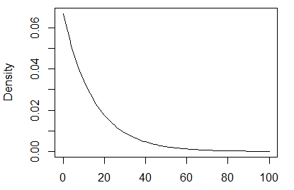
Figure 1: pdf of exponential(1/15)
We can use the rexp() function in R to draw a random sample from an exponential distribution.
data.exp = rexp(100, rate = 1/15)     #draw random sample from exponential(lambda=1/15) distn
qqnorm(data.exp); qqline(data.exp)
_____________________________________________________
Pause for Reflection #5
Why does the normal quantile plot for the exponential data indicate that it is not normal? Support this conclusion by looking at a histogram of data.exp.
_____________________________________________________
Sample Mean from Normal Population: Let's now return to exploring the fact that when sampling from a normally distributed population, the sample mean will also be normally distributed. The following code selects 1000 random samples of size \(n=100\) from a \(N(85,7)\) distribution, computes the mean of each sample, and stores this mean in the vector Xbar. It has been provided in your lab notebook.
Xbar = numeric(1000)
for (i in 1:1000)
{
  x = rnorm(100, 85, 7)
  Xbar[i] = mean(x)
}
hist(Xbar)
qqnorm(Xbar); qqline(Xbar)
_____________________________________________________
Pause for Reflection #6
See how close the simulation-based mean and standard deviation of the sampling distribution for the sample mean are to what the above fact claims they are. In other words, compare the simulated values
mean(Xbar)
sd(Xbar)
to the theoretical values (which you need to compute)
\(\text{E}[\bar{X}] = \mu \quad\) and \(\text{SD}(\bar{X}) = \displaystyle{\sqrt{\frac{\sigma^2}{n}} = \frac{\sigma}{\sqrt{n}}}.\)
Note that the simulated data were random samples of size 100 drawn from a normal distribution with mean 85 and standard deviation 7. Record the results in your lab notebook.
_____________________________________________________
Sample Mean from Non-Normal Population: It turns out that even if the distribution the random samples are taken from is not normal, the sampling distribution of the sample mean is still approximately normal.
To demonstrate this, let's simulate the sampling distribution for the sample mean of random samples from an exponential distribution with mean 15. We can simulate the sampling distribution of a sample mean from this exponential distribution in the same way as we did above for the normal distribution. The following code has been provided in your lab notebook.
Xbar.exp = numeric(1000)
for (i in 1:1000)
{
  x = rexp(100, rate = 1/15)
  Xbar.exp[i] = mean(x)
}
hist(Xbar.exp)
qqnorm(Xbar.exp); qqline(Xbar.exp)
mean(Xbar.exp)
sd(Xbar.exp)
In contrast to the highly skewed distribution of the population (seen in Figure 1 above), the sampling distribution of \(\bar{X}\) is nearly bell shaped, with the normal quantile plot only indicating a hint of skewness.
_____________________________________________________
Pause for Reflection #7
We know that the mean of \(\bar{X}\) should be equal to the mean of the population, which in this case we know to be 15. Does the mean obtained by your simulation approximate this reasonably well?
Note that for an exponential distribution the standard deviation is also given by \(1/\lambda\). Using this, compare the estimated standard deviation of the sampling distribution for \(\bar{X}\) to the theoretical standard deviation:
\(\displaystyle{\frac{\sigma}{\sqrt{n}} = \frac{15}{\sqrt{100}} = 1.5}\).
Record the results of the above in your lab notebook.
_____________________________________________________
Central Limit Theorem (CLT): The reason that the sampling distribution of the sample mean for random samples from non-normal distributions is approximately normal follows from the CLT.
Central Limit Theorem (CLT)
Let \(X_1, \ldots, X_n\) be a random sample from a population with mean \(\mu\) and variance \(\sigma^2\). Then, for any constant \(z\in\mathbb{R}\),
\(\displaystyle{\lim_{n\to\infty} P\left( \frac{\bar{X} - \mu}{\sigma/\sqrt{n}} \leq z\right) = \Phi(z)},\)
where \(\Phi\) denotes the cdf of the standard normal distribution.
The CLT means that for \(n\) "sufficiently large", the sampling distribution of \(\bar{X}\) is approximately normal with mean \(\mu\) and standard deviation \(\sigma/\sqrt{n}\), regardless of the distribution from which the sample was drawn. Thus, the standardized random variable
\(\displaystyle{Z= \frac{\bar{X} - \mu}{\sigma/\sqrt{n}} = \frac{\bar{X} -\text{E}[\bar{X}]}{\text{SD}(\bar{X})}}\)
is approximately normal with mean 0 and standard deviation 1.
_____________________________________________________
Pause for Reflection #8
Return to the simulated sampling distribution of \(\bar{X}\)for a sample from an exponential population with mean 15. We can now use the CLT estimate the probability \(P(\bar{X} > 18)\), as follows:
\(\displaystyle{P(\bar{X} > 18) = P\left( \frac{\bar{X} - 15}{1.5} > \frac{18 - 15}{1.5}\right) \approx P(Z > 2)}, \) where\( Z\sim N(0,1)\).
In your lab notebook, explain how the CLT is being used in the above equation.
We can calculate normal probabilities in R using the function pnorm(). So, \(P(Z>2)\) is given by
pnorm(2, 0, 1, lower.tail=FALSE)
Compare this to the proportion of simulated sample means that were above 18 using the following:
sum(Xbar.exp > 18)/1000
Are the probability given by the CLT and the proportion from the simulation close?
_____________________________________________________