
Lab 10: Simple Linear Regression
- Page ID
- 9053
\( \newcommand{\vecs}[1]{\overset { \scriptstyle \rightharpoonup} {\mathbf{#1}} } \)
\( \newcommand{\vecd}[1]{\overset{-\!-\!\rightharpoonup}{\vphantom{a}\smash {#1}}} \)
\( \newcommand{\dsum}{\displaystyle\sum\limits} \)
\( \newcommand{\dint}{\displaystyle\int\limits} \)
\( \newcommand{\dlim}{\displaystyle\lim\limits} \)
\( \newcommand{\id}{\mathrm{id}}\) \( \newcommand{\Span}{\mathrm{span}}\)
( \newcommand{\kernel}{\mathrm{null}\,}\) \( \newcommand{\range}{\mathrm{range}\,}\)
\( \newcommand{\RealPart}{\mathrm{Re}}\) \( \newcommand{\ImaginaryPart}{\mathrm{Im}}\)
\( \newcommand{\Argument}{\mathrm{Arg}}\) \( \newcommand{\norm}[1]{\| #1 \|}\)
\( \newcommand{\inner}[2]{\langle #1, #2 \rangle}\)
\( \newcommand{\Span}{\mathrm{span}}\)
\( \newcommand{\id}{\mathrm{id}}\)
\( \newcommand{\Span}{\mathrm{span}}\)
\( \newcommand{\kernel}{\mathrm{null}\,}\)
\( \newcommand{\range}{\mathrm{range}\,}\)
\( \newcommand{\RealPart}{\mathrm{Re}}\)
\( \newcommand{\ImaginaryPart}{\mathrm{Im}}\)
\( \newcommand{\Argument}{\mathrm{Arg}}\)
\( \newcommand{\norm}[1]{\| #1 \|}\)
\( \newcommand{\inner}[2]{\langle #1, #2 \rangle}\)
\( \newcommand{\Span}{\mathrm{span}}\) \( \newcommand{\AA}{\unicode[.8,0]{x212B}}\)
\( \newcommand{\vectorA}[1]{\vec{#1}} % arrow\)
\( \newcommand{\vectorAt}[1]{\vec{\text{#1}}} % arrow\)
\( \newcommand{\vectorB}[1]{\overset { \scriptstyle \rightharpoonup} {\mathbf{#1}} } \)
\( \newcommand{\vectorC}[1]{\textbf{#1}} \)
\( \newcommand{\vectorD}[1]{\overrightarrow{#1}} \)
\( \newcommand{\vectorDt}[1]{\overrightarrow{\text{#1}}} \)
\( \newcommand{\vectE}[1]{\overset{-\!-\!\rightharpoonup}{\vphantom{a}\smash{\mathbf {#1}}}} \)
\( \newcommand{\vecs}[1]{\overset { \scriptstyle \rightharpoonup} {\mathbf{#1}} } \)
\(\newcommand{\longvect}{\overrightarrow}\)
\( \newcommand{\vecd}[1]{\overset{-\!-\!\rightharpoonup}{\vphantom{a}\smash {#1}}} \)
\(\newcommand{\avec}{\mathbf a}\) \(\newcommand{\bvec}{\mathbf b}\) \(\newcommand{\cvec}{\mathbf c}\) \(\newcommand{\dvec}{\mathbf d}\) \(\newcommand{\dtil}{\widetilde{\mathbf d}}\) \(\newcommand{\evec}{\mathbf e}\) \(\newcommand{\fvec}{\mathbf f}\) \(\newcommand{\nvec}{\mathbf n}\) \(\newcommand{\pvec}{\mathbf p}\) \(\newcommand{\qvec}{\mathbf q}\) \(\newcommand{\svec}{\mathbf s}\) \(\newcommand{\tvec}{\mathbf t}\) \(\newcommand{\uvec}{\mathbf u}\) \(\newcommand{\vvec}{\mathbf v}\) \(\newcommand{\wvec}{\mathbf w}\) \(\newcommand{\xvec}{\mathbf x}\) \(\newcommand{\yvec}{\mathbf y}\) \(\newcommand{\zvec}{\mathbf z}\) \(\newcommand{\rvec}{\mathbf r}\) \(\newcommand{\mvec}{\mathbf m}\) \(\newcommand{\zerovec}{\mathbf 0}\) \(\newcommand{\onevec}{\mathbf 1}\) \(\newcommand{\real}{\mathbb R}\) \(\newcommand{\twovec}[2]{\left[\begin{array}{r}#1 \\ #2 \end{array}\right]}\) \(\newcommand{\ctwovec}[2]{\left[\begin{array}{c}#1 \\ #2 \end{array}\right]}\) \(\newcommand{\threevec}[3]{\left[\begin{array}{r}#1 \\ #2 \\ #3 \end{array}\right]}\) \(\newcommand{\cthreevec}[3]{\left[\begin{array}{c}#1 \\ #2 \\ #3 \end{array}\right]}\) \(\newcommand{\fourvec}[4]{\left[\begin{array}{r}#1 \\ #2 \\ #3 \\ #4 \end{array}\right]}\) \(\newcommand{\cfourvec}[4]{\left[\begin{array}{c}#1 \\ #2 \\ #3 \\ #4 \end{array}\right]}\) \(\newcommand{\fivevec}[5]{\left[\begin{array}{r}#1 \\ #2 \\ #3 \\ #4 \\ #5 \\ \end{array}\right]}\) \(\newcommand{\cfivevec}[5]{\left[\begin{array}{c}#1 \\ #2 \\ #3 \\ #4 \\ #5 \\ \end{array}\right]}\) \(\newcommand{\mattwo}[4]{\left[\begin{array}{rr}#1 \amp #2 \\ #3 \amp #4 \\ \end{array}\right]}\) \(\newcommand{\laspan}[1]{\text{Span}\{#1\}}\) \(\newcommand{\bcal}{\cal B}\) \(\newcommand{\ccal}{\cal C}\) \(\newcommand{\scal}{\cal S}\) \(\newcommand{\wcal}{\cal W}\) \(\newcommand{\ecal}{\cal E}\) \(\newcommand{\coords}[2]{\left\{#1\right\}_{#2}}\) \(\newcommand{\gray}[1]{\color{gray}{#1}}\) \(\newcommand{\lgray}[1]{\color{lightgray}{#1}}\) \(\newcommand{\rank}{\operatorname{rank}}\) \(\newcommand{\row}{\text{Row}}\) \(\newcommand{\col}{\text{Col}}\) \(\renewcommand{\row}{\text{Row}}\) \(\newcommand{\nul}{\text{Nul}}\) \(\newcommand{\var}{\text{Var}}\) \(\newcommand{\corr}{\text{corr}}\) \(\newcommand{\len}[1]{\left|#1\right|}\) \(\newcommand{\bbar}{\overline{\bvec}}\) \(\newcommand{\bhat}{\widehat{\bvec}}\) \(\newcommand{\bperp}{\bvec^\perp}\) \(\newcommand{\xhat}{\widehat{\xvec}}\) \(\newcommand{\vhat}{\widehat{\vvec}}\) \(\newcommand{\uhat}{\widehat{\uvec}}\) \(\newcommand{\what}{\widehat{\wvec}}\) \(\newcommand{\Sighat}{\widehat{\Sigma}}\) \(\newcommand{\lt}{<}\) \(\newcommand{\gt}{>}\) \(\newcommand{\amp}{&}\) \(\definecolor{fillinmathshade}{gray}{0.9}\)Objectives:
1. Use R to create scatterplots and calculate covariance and correlation.
2. Use linear functions to model relationships between quantitative variables.
Definitions:
- response (dependent) variable
- explanatory/predictor (independent) variable
- scatterplot
- covariance
- correlation
- residual
- RSS: residual sum or squares
- least squares line (or regression line)
Introduction:
Up to this point, our study of statistics has focused on using sample statistics to estimate population parameters. We have seen how to use those estimates to test claims about population parameters. Another use for statistics is to make predictions about parameter values. For example, suppose you find a footprint at the scene of a crime, can the corresponding shoe size be used to make a prediction about the height of the person that left it? In this context, variables now have different roles. There is a response variable, which is the variable that we want to predict (e.g., height), and a predictor variable (also called an explanatory variable), which is used to make the prediction (e.g., shoe size). Furthermore, data come in pairs of observations for both the response and predictor variables. The goal is to develop a model for the relationship between the predictor and response variables. This model can then be used to make predictions. In this lab, we will see how to create a linear model from sample data in order to make predictions. Before we look at developing a model, we review tools for visualizing and quantifying the relationship between variables.
Activities:
Getting Organized: If you are already organized, and remember the basic protocol from previous labs, you can skip this section.
Navigate to your class folder structure. Within your "Labs" folder make a subfolder called "Lab10". Next, download the lab notebook .Rmd file for this lab from Blackboard and save it in your "Lab10" folder. You will be working with the BodyMeasures.csv data set on this lab. You should download the data file into your "Lab10" folder from Blackboard.
Within RStudio, navigate to your "Lab10" folder via the file browser in the lower right pane and then click "More > Set as working directory". Get set to write your observations and R commands in an R Markdown file by opening the "lab10_notebook.Rmd" file in RStudio. Remember to add your name as the author in line 3 of the document. For this lab, enter all of your commands into code chunks in the lab notebook. You can still experiment with code in an R script, if you want. To set up an R Script in RStudio, in the upper left corner click “File > New File > R script”. A new tab should open up in the upper left pane of RStudio.
Scatterplots: The simplest graph for displaying two quantitative variables simultaneously is a scatterplot, which uses the vertical axis for one of the variables and the horizontal axis for the other variable. For each observational pair, a dot is placed at the point with coordinates given by the pair of observations. The convention is to place the response variable on the vertical \(y\)-axis and the predictor variable on the horizontal \(x\)-axis.
For example, consider the file BodyMeasures.csv, which contains that data we collected in class last week on shoe size and height. Suppose we are interested in predicting an individual's height given their shoe size.
_____________________________________________________
Pause for Reflection #1:
State the predictor (\(x\)) and response (\(y\)) variables in the BodyMeasures data set.
_____________________________________________________
The plot() function in R is used to make scatterplots. Type the following code in a code chunk in your notebook to create a scatterplot of the BodyMeasures data. Note that the text() function is used to label points in the scatterplot, which emphasizes that the data set consists of pairs of observations. You can comment it out if it makes the resulting plot difficult to analyze.
data = read.csv("BodyMeasures.csv")
shoe = data$Shoe
height = data$Height

plot(shoe, height, xlab = "shoe size", ylab = "height (in.)",
     main = "Scatterplot of shoe size vs. height")

text(shoe, height, labels = data$ID, pos = 2)     # labels points in plot with ID number
                                                  # pos = 2 places labels to left of points
_____________________________________________________
Pause for Reflection #2:
Use the scatterplot you created to answer the following:
- How would you describe the direction and strength of the association between shoe size and height.
- Does the relationship between shoe size and height appear to be linear?
_____________________________________________________
Covariance & Correlation: We defined two numeric measures in class last week that can be used to quantify the strength of a linear relationship between two numeric variables:
covariance: Cov(\(X, Y\)) = E[(\(X - \mu_X)(Y - \mu_Y)\)]
correlation: \(\rho(X, Y) = \displaystyle \frac{\text{Cov}(X, Y)}{\sigma_X\sigma_Y}\)
The above formulas give the theoretical values of covariance and correlation, i.e. the values if we knew the probability distributions of variables \(X\) and \(Y\), as well as the population means and standard deviations. Since we will most likely not have such information, we estimate covariance and correlation using sample data.
The sample correlation, denoted \(r\), for data \((x_1, y_1), \ldots, (x_n, y_n)\), is calculated using
$$r = \frac{\displaystyle{(1/n)\sum^n_{i=1} (x_i - \bar{x})(y_i - \bar{y})}}{\displaystyle{\sqrt{(1/n)\sum^n_{i=1} (x_i - \bar{x})^2}\sqrt{(1/n)\sum^n_{i=1} (y_i - \bar{y})^2}}}$$
Thankfully, there are functions in R to calculate the covariance and correlation for sample data:
cov(shoe, height)     # sample covariance
cor(shoe, height)     # sample correlation
_____________________________________________________
Pause for Reflection #3:
Convert the height measurements in BodyMeasures from inches to centimeters and recalculate covariance and correlation. (Note that 1 in = 2.54 cm.)
- How do the two covariance values compare? Specifically, is there a way to get the covariance value for the measurements in centimeters from the covariance value in inches?
- Did you get the same value for correlation?
_____________________________________________________
Least-Squares Regression: Whether or not you think the relationship between shoe size and height is linear, we will look at using a linear equation to model it. First, let's see how to use R to construct a "line of best fit" and then we will talk about how that line is actually calculated.
The function lm() in R is used to construct a linear model from sample data. Type the following code in your lab notebook:
lin.reg = lm(height ~ shoe) # list the response first, then the predictor
Once the linear model is fit, we can visualize it in the scatterplot with the following:
plot(shoe, height, xlab = "shoe size", ylab = "height (in.)",
     main = "Scatterplot of shoe size vs. height")
abline(lin.reg, col="orange") # plot the line of best fit in orange
The equation of a generic line can be written as \(\hat{y} = a + bx\), where \(y\) denotes the response variable and \(x\) denotes the predictor variable. In this case, \(x\) represents shoe size and \(y\) represents height, and it is good form to use variable names in the equation. The caret on the \(y\) (read as "y-hat") indicates that its values are predicted, not actual, heights. The symbol \(a\) represents the value of the y-intercept of the line, and \(b\) represents the value of the slope of the line. The slope is the coefficient on \(x\) in the linear model. Typing the stored linear model into R displays the value of \(a\) and \(b\) for the linear model fit to the BodyMeasures data.
lin.reg
_____________________________________________________
Pause for Reflection #4:
- Identify the values of \(a\) and \(b\) for the line of best fit relating shoe size to height.
- Write the equation of the line of best fit using the format \(\hat{y} = a + bx\), but replace \(x\) and \(y\) with the variable names.
_____________________________________________________
What do we mean by "best"? In most statistical applications, we pick the line \(\hat{y} = a + bx\) to make the vertical distances from observations to the line as small as possible, as shown in Figure 1 below. The reason for using vertical distances is that we use \(x\), the predictor variable, to predict or explain \(y\), the response variable, and we try to make the prediction errors as small as possible.
The prediction errors are referred to as residuals. A residual is the difference between the observed \(y\) value and the \(y\) value predicted by the linear model for the corresponding \(x\) value:
residual = \(y - \hat{y}\)
The line of best fit is found by minimizing the residual sum of squares (RSS). The line that achieves the exact minimum value of RSS is called the least squares line, or the regression line.
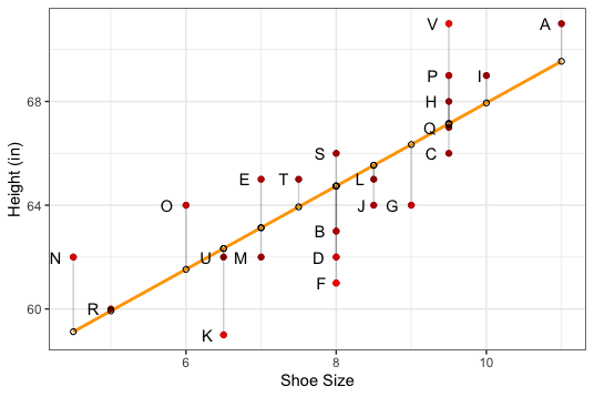
Figure 1: Least Squares Regression Line with Residuals
_____________________________________________________
Pause for Reflection #5:
- Calculate the residual for the observation labeled C in the BodyMeasures data set. To do this, first use the least squares regression line to find the predicted height for C. Note that you found the equation of the least squares regression line in Reflection #4.
- In Figure 1, what is the ID with the largest residual? What is the ID of the smallest residual (in absolute value)?
_____________________________________________________
Pause for Reflection #6:
- Use the least squares regression line to predict the height of someone whose shoe size is 8.
- Use the least squares regression line to predict the height of someone whose shoe size is 9.
- By how much do these predictions differ? Does this number look familiar? Explain.
- What height would the least squares regression line predict for a person with a shoe size of 0? Does this make sense? Explain.
_____________________________________________________