
3.6: Expected Value of Discrete Random Variables
- Page ID
- 4372

\( \newcommand{\vecs}[1]{\overset { \scriptstyle \rightharpoonup} {\mathbf{#1}} } \)
\( \newcommand{\vecd}[1]{\overset{-\!-\!\rightharpoonup}{\vphantom{a}\smash {#1}}} \)
\( \newcommand{\id}{\mathrm{id}}\) \( \newcommand{\Span}{\mathrm{span}}\)
( \newcommand{\kernel}{\mathrm{null}\,}\) \( \newcommand{\range}{\mathrm{range}\,}\)
\( \newcommand{\RealPart}{\mathrm{Re}}\) \( \newcommand{\ImaginaryPart}{\mathrm{Im}}\)
\( \newcommand{\Argument}{\mathrm{Arg}}\) \( \newcommand{\norm}[1]{\| #1 \|}\)
\( \newcommand{\inner}[2]{\langle #1, #2 \rangle}\)
\( \newcommand{\Span}{\mathrm{span}}\)
\( \newcommand{\id}{\mathrm{id}}\)
\( \newcommand{\Span}{\mathrm{span}}\)
\( \newcommand{\kernel}{\mathrm{null}\,}\)
\( \newcommand{\range}{\mathrm{range}\,}\)
\( \newcommand{\RealPart}{\mathrm{Re}}\)
\( \newcommand{\ImaginaryPart}{\mathrm{Im}}\)
\( \newcommand{\Argument}{\mathrm{Arg}}\)
\( \newcommand{\norm}[1]{\| #1 \|}\)
\( \newcommand{\inner}[2]{\langle #1, #2 \rangle}\)
\( \newcommand{\Span}{\mathrm{span}}\) \( \newcommand{\AA}{\unicode[.8,0]{x212B}}\)
\( \newcommand{\vectorA}[1]{\vec{#1}} % arrow\)
\( \newcommand{\vectorAt}[1]{\vec{\text{#1}}} % arrow\)
\( \newcommand{\vectorB}[1]{\overset { \scriptstyle \rightharpoonup} {\mathbf{#1}} } \)
\( \newcommand{\vectorC}[1]{\textbf{#1}} \)
\( \newcommand{\vectorD}[1]{\overrightarrow{#1}} \)
\( \newcommand{\vectorDt}[1]{\overrightarrow{\text{#1}}} \)
\( \newcommand{\vectE}[1]{\overset{-\!-\!\rightharpoonup}{\vphantom{a}\smash{\mathbf {#1}}}} \)
\( \newcommand{\vecs}[1]{\overset { \scriptstyle \rightharpoonup} {\mathbf{#1}} } \)
\( \newcommand{\vecd}[1]{\overset{-\!-\!\rightharpoonup}{\vphantom{a}\smash {#1}}} \)
\(\newcommand{\avec}{\mathbf a}\) \(\newcommand{\bvec}{\mathbf b}\) \(\newcommand{\cvec}{\mathbf c}\) \(\newcommand{\dvec}{\mathbf d}\) \(\newcommand{\dtil}{\widetilde{\mathbf d}}\) \(\newcommand{\evec}{\mathbf e}\) \(\newcommand{\fvec}{\mathbf f}\) \(\newcommand{\nvec}{\mathbf n}\) \(\newcommand{\pvec}{\mathbf p}\) \(\newcommand{\qvec}{\mathbf q}\) \(\newcommand{\svec}{\mathbf s}\) \(\newcommand{\tvec}{\mathbf t}\) \(\newcommand{\uvec}{\mathbf u}\) \(\newcommand{\vvec}{\mathbf v}\) \(\newcommand{\wvec}{\mathbf w}\) \(\newcommand{\xvec}{\mathbf x}\) \(\newcommand{\yvec}{\mathbf y}\) \(\newcommand{\zvec}{\mathbf z}\) \(\newcommand{\rvec}{\mathbf r}\) \(\newcommand{\mvec}{\mathbf m}\) \(\newcommand{\zerovec}{\mathbf 0}\) \(\newcommand{\onevec}{\mathbf 1}\) \(\newcommand{\real}{\mathbb R}\) \(\newcommand{\twovec}[2]{\left[\begin{array}{r}#1 \\ #2 \end{array}\right]}\) \(\newcommand{\ctwovec}[2]{\left[\begin{array}{c}#1 \\ #2 \end{array}\right]}\) \(\newcommand{\threevec}[3]{\left[\begin{array}{r}#1 \\ #2 \\ #3 \end{array}\right]}\) \(\newcommand{\cthreevec}[3]{\left[\begin{array}{c}#1 \\ #2 \\ #3 \end{array}\right]}\) \(\newcommand{\fourvec}[4]{\left[\begin{array}{r}#1 \\ #2 \\ #3 \\ #4 \end{array}\right]}\) \(\newcommand{\cfourvec}[4]{\left[\begin{array}{c}#1 \\ #2 \\ #3 \\ #4 \end{array}\right]}\) \(\newcommand{\fivevec}[5]{\left[\begin{array}{r}#1 \\ #2 \\ #3 \\ #4 \\ #5 \\ \end{array}\right]}\) \(\newcommand{\cfivevec}[5]{\left[\begin{array}{c}#1 \\ #2 \\ #3 \\ #4 \\ #5 \\ \end{array}\right]}\) \(\newcommand{\mattwo}[4]{\left[\begin{array}{rr}#1 \amp #2 \\ #3 \amp #4 \\ \end{array}\right]}\) \(\newcommand{\laspan}[1]{\text{Span}\{#1\}}\) \(\newcommand{\bcal}{\cal B}\) \(\newcommand{\ccal}{\cal C}\) \(\newcommand{\scal}{\cal S}\) \(\newcommand{\wcal}{\cal W}\) \(\newcommand{\ecal}{\cal E}\) \(\newcommand{\coords}[2]{\left\{#1\right\}_{#2}}\) \(\newcommand{\gray}[1]{\color{gray}{#1}}\) \(\newcommand{\lgray}[1]{\color{lightgray}{#1}}\) \(\newcommand{\rank}{\operatorname{rank}}\) \(\newcommand{\row}{\text{Row}}\) \(\newcommand{\col}{\text{Col}}\) \(\renewcommand{\row}{\text{Row}}\) \(\newcommand{\nul}{\text{Nul}}\) \(\newcommand{\var}{\text{Var}}\) \(\newcommand{\corr}{\text{corr}}\) \(\newcommand{\len}[1]{\left|#1\right|}\) \(\newcommand{\bbar}{\overline{\bvec}}\) \(\newcommand{\bhat}{\widehat{\bvec}}\) \(\newcommand{\bperp}{\bvec^\perp}\) \(\newcommand{\xhat}{\widehat{\xvec}}\) \(\newcommand{\vhat}{\widehat{\vvec}}\) \(\newcommand{\uhat}{\widehat{\uvec}}\) \(\newcommand{\what}{\widehat{\wvec}}\) \(\newcommand{\Sighat}{\widehat{\Sigma}}\) \(\newcommand{\lt}{<}\) \(\newcommand{\gt}{>}\) \(\newcommand{\amp}{&}\) \(\definecolor{fillinmathshade}{gray}{0.9}\)In this section, and the next, we look at various numerical characteristics of discrete random variables. These give us a way of classifying and comparing random variables.
Expected Value of Discrete Random Variables
We begin with the formal definition.
Definition \(\PageIndex{1}\)
If \(X\) is a discrete random variable with possible values \(x_1, x_2, \ldots, x_i, \ldots\), and probability mass function \(p(x)\), then the expected value (or mean) of \(X\) is denoted \(\text{E}[X]\) and given by
$$\text{E}[X] = \sum_i x_i\cdot p(x_i).\label{expvalue}$$
The expected value of \(X\) may also be denoted as \(\mu_X\) or simply \(\mu\) if the context is clear.
The expected value of a random variable has many interpretations. First, looking at the formula in Definition 3.6.1 for computing expected value (Equation \ref{expvalue}), note that it is essentially a weighted average. Specifically, for a discrete random variable, the expected value is computed by "weighting'', or multiplying, each value of the random variable, \(x_i\), by the probability that the random variable takes that value, \(p(x_i)\), and then summing over all possible values. This interpretation of the expected value as a weighted average explains why it is also referred to as the mean of the random variable.
The expected value of a random variable is also interpreted as the long-run value of the random variable. In other words, if we repeat the underlying random experiment several times and take the average of the values of the random variable corresponding to the outcomes, we would get the expected value, approximately. (Note: This interpretation of expected value is similar to the relative frequency approximation for probability discussed in Section 1.2.) Again, we see that the expected value is related to an average value of the random variable. Given the interpretation of the expected value as an average, either "weighted'' or "long-run'', the expected value is often referred to as a measure of center of the random variable.
Finally, the expected value of a random variable has a graphical interpretation. The expected value gives the center of mass of the probability mass function, which the following example demonstrates.
Example \(\PageIndex{1}\)
Consider again the context of Example 1.1.1, where we recorded the sequence of heads and tails in two tosses of a fair coin. In Example 3.1.1 we defined the discrete random variable \(X\) to denote the number of heads obtained. In Example 3.2.2 we found the pmf of \(X\). We now apply Equation \ref{expvalue} from Definition 3.6.1 and compute the expected value of \(X\):
\begin{align*}
\text{E}[X] &= 0\cdot p(0) + 1\cdot p(1) + 2\cdot p(2) \\
&= 0\cdot(0.25) + 1\cdot(0.5) + 2\cdot(0.25) \\
&= 0.5 + 0.5 = 1.
\end{align*} Thus, we expect that the number of heads obtained in two tosses of a fair coin will be 1 in the long-run or on average. Figure 1 demonstrates the graphical representation of the expected value as the center of mass of the probability mass function.
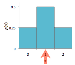
Figure 1: Histogram of \(X\). The red arrow represents the center of mass, or the expected value of \(X\)
Example \(\PageIndex{2}\)
Suppose we toss a fair coin three times and define the random variable \(X\) to be our winnings on a single play of a game where
- we win $\(x\) if the first heads is on the \(x^{th}\) toss, for \(x=1,2,3\),
- and we lose $1 if we get no heads in all three tosses.
Then \(X\) is a discrete random variable, with possible values \(x=-1,1,2,3\), and pmf given by the following table:
| \(x\) | \(p(x) = P(X=x)\) |
| \(-1\) | \(\frac{1}{8}\) |
| \(1\) | \(\frac{1}{2}\) |
| \(2\) | \(\frac{1}{4}\) |
| \(3\) | \(\frac{1}{8}\) |
Applying Definition 3.6.1, we find \begin{align*}
\text{E}[X] &= \sum_i x_i\cdot p(x_i) \\
&= (-1)\cdot\frac{1}{8} + 1\cdot\frac{1}{2} + 2\cdot\frac{1}{4} + 3\cdot\frac{1}{8} = \frac{5}{4} = 1.25.
\end{align*} Thus, the expected winnings for a single play of the game is $1.25. In other words, if we played the game multiple times, we expect the average winnings to be $1.25.
For many of the common probability distributions, the expected value is given by a parameter of the distribution as the next exercise shows for the Poisson distribution.
Exercise \(\PageIndex{1}\)
Suppose the discrete random variable \(X\) has a Poisson distribution with parameter \(\lambda\). Show that \(\text{E}[X] = \lambda\).
- Hint
- Recall from calculus the series expansion: \(\displaystyle{e^y = \sum^{\infty}_{x=1} \frac{y^{x-1}}{(x-1)!}}\)
- Answer
-
First, recall that the pmf for Poisson distribution is \(\displaystyle{p(x) = \frac{e^{-\lambda}\lambda^{x}}{x!}}\), for \(x=0, 1, \ldots\). Then, we apply Definition 3.6.1, giving us
\begin{align*}
\text{E}[X] &= \sum^{\infty}_{x=0} x\cdot p(x)\\
&= \sum^{\infty}_{x=0} x\cdot\frac{e^{-\lambda}\lambda^{x}}{x!} \quad\text{(note that the}\ x=0\ \text{term is 0, so we drop it from the sum)}\\
&= \sum^{\infty}_{\textcolor{orange}{x=1}} x\cdot \frac{e^{-\lambda}\textcolor{blue}{\lambda^{x}}}{\textcolor{red}{x!}} = \sum^{\infty}_{x=1} x\cdot \frac{e^{-\lambda}\textcolor{blue}{\lambda\cdot\lambda^{x-1}}}{\textcolor{red}{x\cdot(x-1)!}} \\
&= e^{-\lambda}\cdot \lambda \sum^{\infty}_{x=1} \frac{\lambda^{x-1}}{(x-1)!}\\
&= e^{-\lambda}\cdot \lambda \cdot e^{\lambda} \quad\quad\text{(here we used the series expansion of}\ e^y)\\
&= \lambda\\
\end{align*} as needed.
The expected value may not be exactly equal to a parameter of the probability distribution, but rather it may be a function of the parameters. The following table gives the expected value for each of the common discrete distributions we considered earlier. We will see later (Section 3.8) how to derive these results using a technique involving moment-generating functions.
| Distribution | Expected Value |
| Bernoulli(\(p\)) | \(p\) |
| binomial(\(n, p\)) | \(np\) |
| hypergeometric(\(N, n, m\)) | \(\frac{nm}{N}\) |
| geometric(\(p\)) | \(\frac{1}{p}\) |
| negative binomial(\(r, p\)) | \(\frac{r}{p}\) |
| Poisson(\(\lambda\)) | \(\lambda\) |
Expected Value of Functions of Random Variables
In many applications, we may not be interested in the value of a random variable itself, but rather in a function applied to the random variable or a collection of random variables. For example, we may be interested in the value of \(X^2\). The following theorems, which we state without proof, demonstrate how to calculate the expected value of functions of random variables.
Theorem \(\PageIndex{1}\)
Let \(X\) be a random variable and let \(g\) be a real-valued function. Define the random variable \(Y = g(X)\).
If \(X\) is a discrete random variable with possible values \(x_1, x_2, \ldots, x_i, \ldots\), and probability mass function \(p(x)\), then the expected value of \(Y\) is given by
$$\text{E}[Y] = \sum_i g(x_i)\cdot p(x_i).\notag$$
To put it simply, Theorem 3.6.1 states that to find the expected value of a function of a random variable, just apply the function to the possible values of the random variable in the definition of expected value. Before stating an important special case of Theorem 3.6.1, a word of caution regarding order of operations. Note that, in general,
$$\text{E}[g(X)] \neq g\left(\text{E}[X]\right)\text{!}\label{caution}$$
For example, \(\text{E}[X^2] \neq (\text{E}[X])^2\), in general. However, as the next theorem states, there are exceptions to Equation \ref{caution}.
Special Case of Theorem 3.6.1
Let \(X\) be a random variable. If \(g\) is a linear function, i.e., \(g(x) = ax + b\), then
$$\text{E}[g(X)] = \text{E}[aX + b] = a\text{E}[X] + b.\notag$$
The above special case is referred to as the linearity of expected value, which implies the following properties of the expected value.
Linearity of Expected Value
Let \(X\) be a random variable, \(c, c_1, c_2\) constants, and \(g, g_1, g_2\) real-valued functions. Then expectiation \(\text{E}[\cdot]\) satisfies the following:
- The expected value of a constant is constant: $$\text{E}[c] = c\notag$$
- Constants can be factored out of expected values: $$\text{E}[cg(X)] = c\text{E}[g(X)]\notag$$
- The expected value of a sum is equal to the sum of expected values: $$\text{E}[c_1g_1(X) + c_2g_2(X)] = c_1\text{E}[g_1(X)] + c_2\text{E}[g_2(X)]\notag$$