7.1: Other Useful Distributions

Last updated
Save as PDF

Page ID: 12778

$ \newcommand{\vecs}[1]{\overset { \scriptstyle \rightharpoonup} {\mathbf{#1}} } $ $ \newcommand{\vecd}[1]{\overset{-\!-\!\rightharpoonup}{\vphantom{a}\smash {#1}}} $$\newcommand{\id}{\mathrm{id}}$ $ \newcommand{\Span}{\mathrm{span}}$ $ \newcommand{\kernel}{\mathrm{null}\,}$ $ \newcommand{\range}{\mathrm{range}\,}$ $ \newcommand{\RealPart}{\mathrm{Re}}$ $ \newcommand{\ImaginaryPart}{\mathrm{Im}}$ $ \newcommand{\Argument}{\mathrm{Arg}}$ $ \newcommand{\norm}[1]{\| #1 \|}$ $ \newcommand{\inner}[2]{\langle #1, #2 \rangle}$ $ \newcommand{\Span}{\mathrm{span}}$ $\newcommand{\id}{\mathrm{id}}$ $ \newcommand{\Span}{\mathrm{span}}$ $ \newcommand{\kernel}{\mathrm{null}\,}$ $ \newcommand{\range}{\mathrm{range}\,}$ $ \newcommand{\RealPart}{\mathrm{Re}}$ $ \newcommand{\ImaginaryPart}{\mathrm{Im}}$ $ \newcommand{\Argument}{\mathrm{Arg}}$ $ \newcommand{\norm}[1]{\| #1 \|}$ $ \newcommand{\inner}[2]{\langle #1, #2 \rangle}$ $ \newcommand{\Span}{\mathrm{span}}$$\newcommand{\AA}{\unicode[.8,0]{x212B}}$

In this section, we introduce three more continuous probability distributions: the chi-squared, $t$, and $F$ distributions. All three of these are very useful in the study of statistics. And we will see that each are built from the normal distribution in some way.

Chi-Squared Distributions

Definition $\PageIndex{1}$

If $Z\sim N(0,1)$, then the probability distribution of $U = Z^2$ is called the chi-squared distribution with $1$ degree of freedom (df) and is denoted $\chi^2_1$.

This definition of the chi-squared distribution with 1 df is stated in terms of a standard normal random variable, which we can relate to any non-standard normal random variable as follows. Let $X\sim N(\mu, \sigma^2)$, then
$$\frac{X-\mu}{\sigma} \sim N(0,1) \quad\Rightarrow\quad \left(\frac{X-\mu}{\sigma}\right)^2 \sim \chi^2_1.\notag$$
We can also extend the definition of a chi-squared distribution to have more than one degree of freedom by simply summing any number of independent $\chi^2_1$ distributed random variables.

Definition $\PageIndex{2}$

If $U_1, U_2, \ldots, U_n$ are independent $\chi^2_1$ random variables, then the probability distribution of $V = U_1 + U_2 + \cdots + U_n$ is called the chi-squared distribution with $n$ degrees of freedom (df) and is denoted $\chi^2_n$.

Note that we could have stated Definition 7.1.2 using a collection of independent, standard normal random variables $Z_1, Z_2, \ldots, Z_n$, since by Definition 7.1.1 the square of each $Z_i^2$ is a $\chi^2_1$ distributed random variable. In other words, the following is another possible definition of the chi-squared distribution with $n$ degrees of freedom:
$$Z_1^2 + Z_2^2 + \cdots + Z_n^2 \sim \chi^2_n \notag$$

Definition 7.1.2 also leads to the following useful property of the chi-squared distribution. Namely, if $X\sim\chi^2_m$ and $Y\sim\chi^2_n$ are independent random variables, then $X+Y\sim\chi^2_{m+n}$. This easily follows from the definition, since every chi-squared distributed random variable is just a sum of independent $\chi^2_1$ random variables, so summing two chi-squared random variables is just one big sum of many $\chi^2_1$ random variables, where the number is given by the sum of the respective degrees of freedom.

While we will not have much reason to use it, the following theorem (stated without proof) provides the explicit formula for the pdf of the chi-squared distribution.

Theorem $\PageIndex{1}$

Let the random variable $V$ have a chi-squared distribution with $n$ degrees of freedom. Then $V$ has pdf given by
$$f(v) = \left\{\begin{array}{l l}
\displaystyle{\frac{1}{\Gamma(n/2)2^{n/2}} v^{n/2-1} e^{-v/2}}, & \text{for}\ v\geq 0, \\
0 & \text{otherwise,}
\end{array}\right. \notag$$

where $\Gamma(n/2)$ is a function (referred to as the gamma function) given by the following integral:
$$\Gamma(n/2) = \int^{\infty}_0 t^{n/2-1}e^{-t}dt. \notag$$

Figure 1: Graph of pdf for $\chi^2(1)$ distribution.

The chi-squared distributions are a special case of the gamma distributions with $\alpha = \frac{n}{2}, \lambda=\frac{1}{2}$, which can be used to establish the following properties of the chi-squared distribution.

Properties of Chi-Squared Distributions

If $V\sim\chi^2_n$, then $V$ has the following properties.

The mean of $V$ is $\text{E}[V] = n$, i.e., the degrees of freedom.
The variance of $V$ is $\text{Var}(V) = 2n$, i.e., twice the degrees of freedom.

Note that there is no closed form equation for the cdf of a chi-squared distribution in general. But programming languages, such as Python and R, have a built-in function to compute chi-squared probabilities.

t Distributions

Definition $\PageIndex{3}$

If $Z\sim N(0,1)$ and $U\sim \chi^2_n$, and $Z$ and $U$ are independent, then the probability distribution of
$$T = \frac{Z}{\sqrt{U/n}}\notag$$
is called the t distribution with $n$ degrees of freedom and is denoted $t_n$.

Like the chi-squared distributions, the $t$ distributions depend on a parameter referred to as the degrees of freedom.

The $t$ distribution behaves in a similar manner to the standard normal distribution, with one main distinction. To see this, consider the graph provided in Figure 2 below, which gives the pdf's for the standard normal distribution and four different $t$ distributions. Note that just like the standard normal distribution, all $t$ distributions have a similarly bell-shaped pdf curve which is centered and symmetric about 0. In fact, the expected value or mean of any random variable with a $t$ distribution is always equal to 0. However, the $t$ distribution does not have the same variance as the standard normal distribution, in fact all $t$ distributions have larger variance than the standard normal, which can be seen in the graph by looking at the "tails" of the pdf's, i.e., the extreme regions far away from the mean. For instance, consider the regions less than $-2$ and greater than $2$. Note that in these regions, there is more area under each of the $t$ distribution pdf curves because each of these curves is above the pdf of the standard normal distribution. Given that there is more area under the $t$ distribution pdf curves in these extreme regions, this implies that there is a higher probability that the value of a random variable with a $t$ distribution would be this far away from the center compared to a standard normal random variable, meaning that there is greater spread in the values from the mean and hence a larger variance for the $t$ distribution. Stated another way, the "tails" of all $t$ distribution pdf's are thicker than the "tails" of the standard normal. We will see in the next section that this aspect of the $t$ distribution is what makes it so useful in the study of statistics.

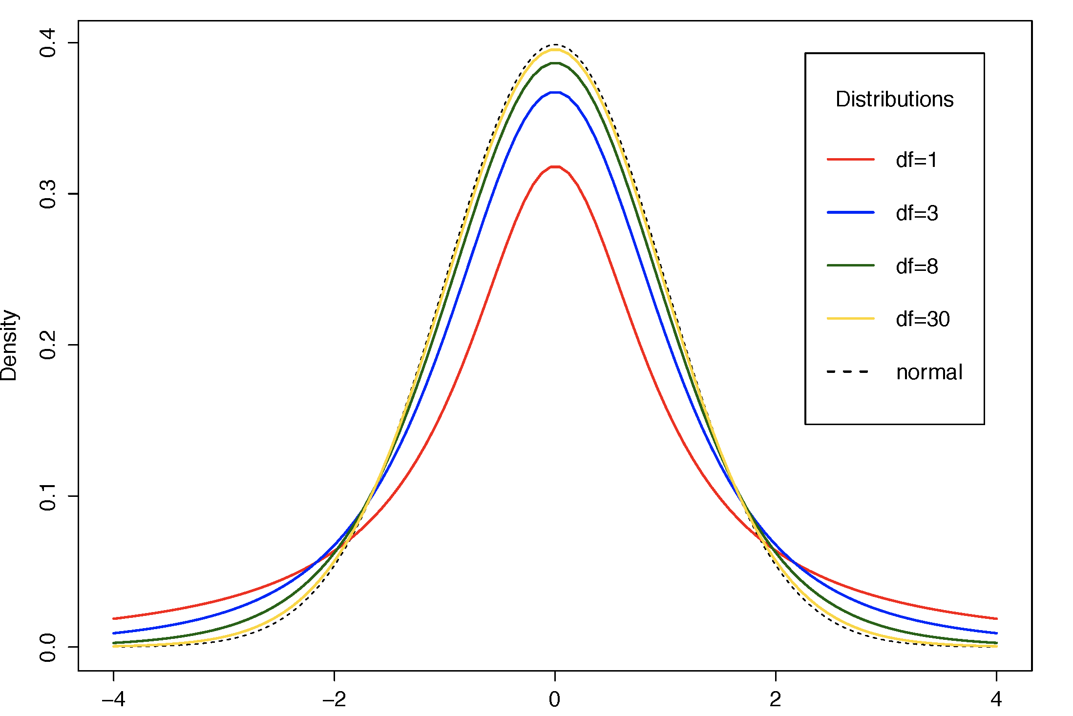
Figure 2: Comparison of $t$ distributions to $N(0,1$ distribution.

One final aspect of the $t$ distribution is to note that as the degrees of freedom increase, the pdf curves approach the standard normal pdf. In Figure 2, consider the red curve, which corresponds to the pdf of a $t_1$ distribution. This pdf is rather different than the standard normal pdf curve (which is the black dashed line): the middle peak is lower and the tails are much thicker. However, if we consider the yellow curve, which corresponds to the pdf of a $t_{30}$ distribution, we see very little difference from the standard normal pdf. Indeed, it is very hard to distinguish those two pdf's in Figure 2. In fact, the $t$ distributions approach the standard normal distribution in the limit as the degrees of freedom approach infinity:
$$t_n \rightarrow N(0,1) \quad\text{as}\ n\rightarrow\infty \notag$$

Again, for completeness more than practical use, we state the following theorem (without proof) which provides the explicit formula for the pdf of the $t$ distribution.

Theorem $\PageIndex{2}$

Let the random variable $T$ have a $t$ distribution with $n$ degrees of freedom. Then $T$ has pdf given by
$$f(t) = \frac{\Gamma\left(\frac{n+1}{2}\right)}{\Gamma(n/2)\sqrt{n\pi}} \left(1 + \frac{t^2}{n}\right)^{-(n+1)/2}, \quad\text{for}\ t\in\mathbb{R}, \notag$$

where $\Gamma$ denotes the gamma function defined in Theorem 7.1.1 above.

F Distributions

Definition $\PageIndex{4}$

If $U\sim\chi^2_m$ and $V\sim\chi^2_n$ are independent random variables, then the probability distribution of
$$W = \frac{U/m}{V/n}\notag$$
is called the F distribution with $m$ and $n$ degree of freedom (df) and is denoted $F_{m,n}$.

Given that the $F$ distribution is built from the ratio of two independent chi-squared distributions, the $F$ distribution has two sets of degrees of freedom. The first set, denoted $m$ in Definition 7.1.4, is referred to as the numerator degrees of freedom, and the second set $n$ is referred to as the denominator degrees of freedom.

The following theorem connects the $t$ distribution to the $F$ distribution.

Theorem $\PageIndex{3}$

If $T\sim t_n$, then $T^2\sim F_{1,n}$.

Proof: By Definition 7.1.3, we know that $T$ can be written as $Z/\sqrt{U/n}$, for independent random variables $Z\sim N(0,1)$ and $U\sim\chi^2_n$. This gives
$$T^2 = \frac{Z^2}{U/n}.\notag$$
Now notice that Definition 7.1.1 states that $Z^2\sim\chi^2_1$, and so $T^2$ is equal to the ratio of two independent chi-squared random variables, each divided by their degrees of freedom. Thus, by Definition 7.1.4, $T^2$ has an $F$ distribution with 1 numerator df and $n$ denominator df.

And finally, we state the explicit formula for the pdf of the $F$ distribution for completeness.

Theorem $\PageIndex{4}$

Let the random variable $W$ have a $F$ distribution with $m$ and $n$ degrees of freedom. Then $W$ has pdf given by
$$f(w) = \frac{\Gamma\left(\frac{m+n}{2}\right)}{\Gamma(m/2)\Gamma(n/2)} \left(\frac{m}{n}\right)^{m/2} w^{\frac{m}{2} - 1} \left(1 + \frac{m}{n}w\right)^{-(m+n)/2}, \quad\text{for}\ w\geq0, \notag$$

where $\Gamma$ denotes the gamma function defined in Theorem 7.1.1 above.

Search

Definition \(\PageIndex{1}\)

Definition \(\PageIndex{2}\)

Theorem \(\PageIndex{1}\)

Properties of Chi-Squared Distributions

Definition \(\PageIndex{3}\)

Theorem \(\PageIndex{2}\)

Definition \(\PageIndex{4}\)

Theorem \(\PageIndex{3}\)

Theorem \(\PageIndex{4}\)