6.2: Sample Mean

Last updated
Save as PDF

Page ID: 12776

$ \newcommand{\vecs}[1]{\overset { \scriptstyle \rightharpoonup} {\mathbf{#1}} } $ $ \newcommand{\vecd}[1]{\overset{-\!-\!\rightharpoonup}{\vphantom{a}\smash {#1}}} $$\newcommand{\id}{\mathrm{id}}$ $ \newcommand{\Span}{\mathrm{span}}$ $ \newcommand{\kernel}{\mathrm{null}\,}$ $ \newcommand{\range}{\mathrm{range}\,}$ $ \newcommand{\RealPart}{\mathrm{Re}}$ $ \newcommand{\ImaginaryPart}{\mathrm{Im}}$ $ \newcommand{\Argument}{\mathrm{Arg}}$ $ \newcommand{\norm}[1]{\| #1 \|}$ $ \newcommand{\inner}[2]{\langle #1, #2 \rangle}$ $ \newcommand{\Span}{\mathrm{span}}$ $\newcommand{\id}{\mathrm{id}}$ $ \newcommand{\Span}{\mathrm{span}}$ $ \newcommand{\kernel}{\mathrm{null}\,}$ $ \newcommand{\range}{\mathrm{range}\,}$ $ \newcommand{\RealPart}{\mathrm{Re}}$ $ \newcommand{\ImaginaryPart}{\mathrm{Im}}$ $ \newcommand{\Argument}{\mathrm{Arg}}$ $ \newcommand{\norm}[1]{\| #1 \|}$ $ \newcommand{\inner}[2]{\langle #1, #2 \rangle}$ $ \newcommand{\Span}{\mathrm{span}}$$\newcommand{\AA}{\unicode[.8,0]{x212B}}$

Suppose we are interested in understanding the mean of some population of values, but do not have full information about the entire population. One approach to solving this problem is to obtain a random sample of a subset of values from the population and consider the mean of the sample. The mean of the sample is referred to as the sample mean. Since the sample is randomly selected, the sample mean may be thought of as a function applied to a collection of random variables.

Example $\PageIndex{1}$

Suppose we want to know the average SAT math score for girls in Indiana. We could randomly select seniors from high schools in the South Bend School Corporation as a sample from all IN girls, and use the mean SAT math score for the South Bend girls as an estimate of the overall mean for IN girls.

The mean of SB girls depends on which sample we randomly select, therefore the sample mean is a random variable.

The probability distribution of the sample mean is referred to as the sampling distribution of the sample mean. The following result, which is a corollary to Sums of Independent Normal Random Variables, indicates how to find the sampling distribution when the population of values follows a normal distribution.

Corollary $\PageIndex{1}$

If $X_1, \ldots, X_n$ represent the values of a random sample from a $N(\mu, \sigma)$ population, then the sample mean
$$\bar{X} = \frac{X_1 + \cdots + X_n}{n} = \sum^n_{i=1} \frac{1}{n}X_i,\notag$$
is normally distributed with mean $\mu$ and standard deviation $\sigma/\sqrt{n}$. In other words, we can write
$$\bar{X}\sim N(\mu, \sigma/\sqrt{n}).\notag$$

Proof

Sample observations are independent when randomly selected. Furthermore, each observation has same distribution as population. $X_1,\cdots,X_n$ represent the observations in the random sample $\Longrightarrow X_1,\cdots, X_n$ are independent and each $X_i\sim N(\mu,\sigma)$
$\bar{X}$ is the sum of independent normally distributed random variables: $$\bar{X} = \frac{X_1+\cdots+X_n}{n} = \frac{X_1}{n}+\frac{X_2}{n}+\cdots+\frac{X_n}{n} = \sum^n_{i=1} \frac{1}{n}X_i \Longrightarrow a_i = \frac{1}{n}, \text{ for } i = 1,\cdots,n\notag$$
By Sums of Independent Normal Random Variables: $\bar{X}\sim N(\mu_{\bar{X}},\sigma_{\bar{X}})$, where

    \begin{align*}
         \mu_{\bar{X}} &= \sum^n_{i=1} \frac{1}{n}\mu = \frac{1}{n}\mu + \cdots + \frac{1}{n}\mu = n\frac{1}{n}\mu = \mu \\
         \sigma_{\bar{X}}^2 &= \sum^n_{i=1}(\frac{1}{n})^2\sigma^2 = n\frac{1}{n^2}\sigma^2 = \frac{\sigma^2}{n}\\
         \Longrightarrow \sigma_{\bar{X}} &= \sqrt{\sigma_{\bar{X}}^2} = \sqrt{\frac{\sigma^2}{n}} = \frac{\sigma}{\sqrt{n}}
    \end{align*}

So $\bar{X}\sim N(\mu,\frac{\sigma}{\sqrt{n}})$.

Example $\PageIndex{2}$

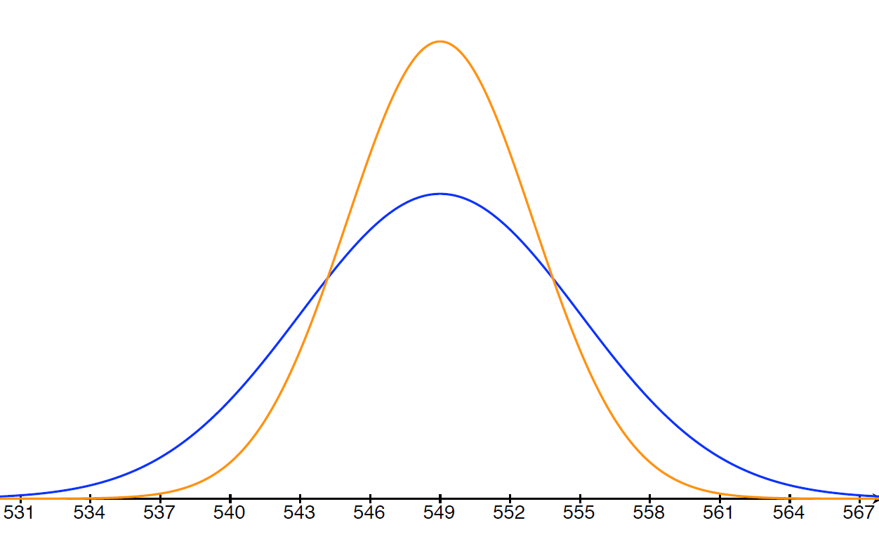
Suppose that SAT math scores for girls in Indiana are assumed to be $N(549, 24)$.

Find and compare the sampling distributions for the sample means from a sample of size $n=16$ and a sample of size $n=36$.

For $n=16: $ sample mean $\displaystyle{\bar{X}\sim\text{ N}\left(549,\frac{24}{\sqrt{16}}=6\right)}$

For $n=36: $ sample mean $\displaystyle{\bar{Y}\sim\text{ N}\left(549,\frac{24}{\sqrt{36}} = 4\right)}$

Let's find the probability that each sample mean will be within 10 points of actual population mean ($\mu = 549$):

$\bar{X}: P(|\bar{X}-\mu|\leq 10) = P(539\leq \bar{X}\leq 559) = \text{normalcdf}(539,559,549,6) = 0.9044$

$\bar{Y}: P(539\leq \bar{Y} \leq 559) = \text{normalcdf}(539,559,549,4) = 0.9876$

Note that the "normalcdf" in the above equations refers to the built-in function on many graphing calculators used to evaluate probabilities for the normal distribution. If you do not have a graphing calculator, do not worry! Many programming languages, such as Python and R, offer built-in functions to evaluate normal probabilities. However, an even simpler option is to use the online normal distribution calculator available at this link.

The following figure gives the plot of the pdf's for the sampling distributions of $\bar{X}$(blue) and $\bar{Y}$(yellow). Note that the spread of the pdf for $\bar{X}$ is larger than for $\bar{Y}$. This is due to the fact that the sample size that $\bar{X}$ is based on is smaller than the sample size for $\bar{Y}$. In other words, the sd of the sample mean is inversely related to the sample size, which can be seen in the formula provided by Corollary 6.2.1 where we see that the sample size occurs in the denominator.

The Central Limit Theorem

We saw that when "sampling'' from a normally distributed population, the sampling distribution of the sample mean is also normal. But what if the population does not follow a normal distribution? What if it is skewed or uniform?

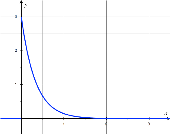
Example $\PageIndex{3}$

Suppose we are interested in the lifetime of a radioactive particle. The probability distribution of such lifetimes can be modeled with an exponential distribution. If $\lambda = 3$, for example, then the pdf is skewed right, because there is a tail of values with very low probabilities off to the right.

Central Limit Theorem

Let $X_1, \ldots, X_n$ be a random sample from any probability distribution with mean $\mu$ and sd $\sigma$. Then as the sample size $n\rightarrow\infty$, the probability distribution of the sample mean approaches the normal distribution. We write:

$$\bar{X} \xrightarrow{d} N(\mu, \sigma/\sqrt{n}), \quad\text{as}\ n\to\infty\label{dlimit}$$
In other words, if $n$ is sufficiently large, we can approximate the sampling distribution of the sample mean as $N(\mu, \sigma/\sqrt{n})$.

Furthermore, $$\frac{\bar{X}-\mu}{\sigma/\sqrt{n}}\approx N(0,1) \text{ as } n\rightarrow \infty\label{clt}$$

The $d$ above the arrow in Equation \ref{dlimit} above stands for distribution and indicates that, as the sample size increases without bound, the limit of the probability distribution of $\bar{X}$ is given by the $N(\mu, \sigma/\sqrt{n})$ distribution. This is referred to as convergence in distribution.

What's "sufficiently large''?

If the distribution of the $X_i$ is symmetric, unimodal or continuous, then a sample size $n$ as small as 4 or 5 yields an adequate approximation.
If the distribution of the $X_i$ is skewed, then a sample size $n$ of at least 25 or 30 yields an adequate approximation.
If the distribution of the $X_i$ is extremely skewed, then you may need an even larger $n$.

The following website provides a simulation of sampling distributions and demonstrates the Central Limit Theorem (link available).

Example $\PageIndex{4}$

Continuing in the context of Example 6.2.3, suppose we sample $n=25$ such radioactive particles. Then the sampling distribution of the mean of the sample is approximated as follows.

Letting $X_1, \ldots, X_{25}$ denote the random sample, we have that each $X_i \sim \text{exponential}(\lambda = 3)$. By the Properties of Exponential Distributions, we know that the mean of an exponential(3) distribution is given by $\mu = \frac{1}{\lambda} = \frac{1}{3}$ and the sd is also $\sigma=\frac{1}{\lambda} = \frac{1}{3}$. Thus, the sampling distribution of the sample mean is $$\bar{X} \sim N\left(\frac{1}{3},\frac{1/3}{\sqrt{25}}\right) \Rightarrow N\left(\frac{1}{3},\frac{1}{15}\right).\notag$$

What is the use of the Central Limit Theorem if we don't know $\mu$, the mean of the population? We can use the CLT to approximate estimation error probabilities: $$P(|\bar{x} - \mu| \leq \varepsilon),\label{error}$$ the probability that $\bar{X}$ is within $\varepsilon$ units of $\mu$. By the Central Limit Theorem and Equation \ref{clt}, we know $$\frac{\bar{X}-\mu}{\sigma/\sqrt{n}}\approx N(0,1).$$ From this fact, we can isolate $\mu$ in the inequality in Equation \ref{error} as follows: $$P(|\bar{X} - \mu| \leq \varepsilon) = P\left(\frac{|\bar{X}-\mu|}{\sigma/\sqrt{n}} \leq \frac{\varepsilon}{\sigma/\sqrt{n}}\right) \approx P\left(|Z|\leq \frac{\varepsilon}{\sigma/\sqrt{n}}\right) = P\left(-\frac{\varepsilon}{\sigma/\sqrt{n}} \leq Z \leq \frac{\varepsilon}{\sigma/\sqrt{n}} \right)$$

Example $\PageIndex{5}$

Now suppose that we do not know the rate at which the radioactive particle of interest decays, i.e., we do not know the mean lifetime of such particles. We can develop a method for approximating the probability that the mean of a sample of size $n=25$ is within $1$ unit of the mean lifetime.

In other words, we want $P(|\bar{X} - \mu| \leq 1)$.

By the Central Limit Theorem and Equation \ref{clt}, we know that $$\frac{\bar{X}-\mu}{\sigma/\sqrt{25}} = \frac{\bar{X}-\mu}{\sigma/5}\approx N(0,1).\notag$$ From this we derive a formula for the desired probability: $$P\left(\frac{\bar{X}-\mu}{\sigma/5} \leq \frac{1}{\sigma/5}\right) \approx P\left(|Z|\leq \frac{5}{\sigma}\right) \notag$$

Search

Corollary \(\PageIndex{1}\)

Central Limit Theorem

Example \(\PageIndex{4}\)

Example \(\PageIndex{5}\)

Example \(\PageIndex{1}\)

Corollary \(\PageIndex{1}\)

Example \(\PageIndex{2}\)

The Central Limit Theorem

Example \(\PageIndex{3}\)

Central Limit Theorem

Example \(\PageIndex{4}\)

Example \(\PageIndex{5}\)