3.2: Probability Mass Functions (PMFs) and Cumulative Distribution Functions (CDFs) for Discrete Random Variables

Since random variables simply assign values to outcomes in a sample space and we have defined probability measures on sample spaces, we can also talk about probabilities for random variables. Specifically, we can compute the probability that a discrete random variable equals a specific value (probability mass function) and the probability that a random variable is less than or equal to a specific value (cumulative distribution function).

Probability Mass Functions (PMFs)

In the following example, we compute the probability that a discrete random variable equals a specific value.

Example \(\PageIndex{1}\)

Continuing in the context of Example 3.1.1, we compute the probability that the random variable \(X\) equals \(1\). There are two outcomes that lead to \(X\) taking the value 1, namely \(ht\) and \(th\). So, the probability that \(X=1\) is given by the probability of the event \({ht, th}\), which is \(0.5\):

$$P(X=1) = P(\{ht, th\}) = \frac{\text{# outcomes in}\ \{ht, th\}}{\text{# outcomes in}\ S} = \frac{2}{4} = 0.5\notag$$

---

In Example 3.2.1, the probability that the random variable \(X\) equals 1, \(P(X=1)\), is referred to as the probability mass function of \(X\) evaluated at 1. In other words, the specific value 1 of the random variable \(X\) is associated with the probability that \(X\) equals that value, which we found to be 0.5. The process of assigning probabilities to specific values of a discrete random variable is what the probability mass function is and the following definition formalizes this.

Definition \(\PageIndex{1}\)

The probability mass function (pmf) (or frequency function) of a discrete random variable \(X\) assigns probabilities to the possible values of the random variable. More specifically, if \(x_1, x_2, \ldots\) denote the possible values of a random variable \(X\), then the probability mass function is denoted as \(p\) and we write
$$p(x_i) = P(X=x_i) = P(\underbrace{\{\omega\in \Omega\ |\ X(s) = x_i\}}_{\text{set of outcomes resulting in}\ X=x_i}).\label{pmf}$$

Note that, in Equation \ref{pmf}, \(p(x_i)\) is shorthand for \(P(X = x_i)\), which represents the probability of the event that the random variable \(X\) equals \(x_i\).

As we can see in Definition 3.2.1, the probability mass function of a random variable \(X\) depends on the probability measure of the underlying sample space \(\Omega\). Thus, pmf's inherit some properties from the axioms of probability (Definition 1.2.1). In fact, in order for a function to be a valid pmf it must satisfy the following properties.

Properties of Probability Mass Functions

Let \(X\) be a discrete random variable with possible values denoted \(x_1, x_2, \ldots, x_i, \ldots\). The probability mass function of \(X\), denoted \(p\), must satisfy the following:

1. \(\displaystyle{\sum_{x_i} p(x_i)} = p(x_1) + p(x_2) + \cdots = 1\)
2. \(p(x_i) \geq 0\), for all \(x_i\)

Furthermore, if \(A\) is a subset of the possible values of \(X\), then the probability that \(X\) takes a value in \(A\) is given by

$$P(X\in A) = \sum_{x_i\in A} p(x_i).\label{3rdprop}$$

Note that the first property of pmf's stated above follows from the first axiom of probability, namely that the probability of the sample space equals \(1\): \(P(\Omega) = 1\). The second property of pmf's follows from the second axiom of probability, which states that all probabilities are non-negative.

We now apply the formal definition of a pmf and verify the properties in a specific context.

Example \(\PageIndex{2}\)

Returning to Example 3.2.1, now using the notation of Definition 3.2.1, we found that the pmf for \(X\) at \(1\) is given by
$$p(1) = P(X=1) = P(\{ht, th\}) = 0.5.\notag$$
Similarly, we find the pmf for \(X\) at the other possible values of the random variable:
\begin{align*}
p(0) &= P(X=0) = P(\{tt\}) = 0.25 \\
p(2) &= P(X=2) = P(\{hh\}) = 0.25
\end{align*}
Note that all the values of \(p\) are positive (second property of pmf's) and \(p(0) + p(1) + p(2) = 1\) (first property of pmf's). Also, we can demonstrate the third property of pmf's (Equation \ref{3rdprop}) by computing the probability that there is at least one heads, i.e., \(X\geq 1\), which we could represent by setting \(A = \{1,2\}\) so that we want the probability that \(X\) takes a value in \(A\):

$$P(X\geq1) = P(X\in A) = \sum_{x_i\in A}p(x_i) = p(1) + p(2) = 0.5 + 0.25 = 0.75\notag$$

---

We can represent probability mass functions numerically with a table, graphically with a histogram, or analytically with a formula. The following example demonstrates the numerical and graphical representations. In the next three sections, we will see examples of pmf's defined analytically with a formula.

Example \(\PageIndex{3}\)

We represent the pmf we found in Example 3.2.2 in two ways below, numerically with a table on the left and graphically with a histogram on the right.

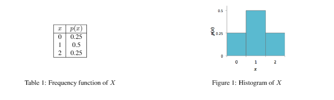
In the histogram in Figure 1, note that we represent probabilities as areas of rectangles. More specifically, each rectangle in the histogram has width \(1\) and height equal to the probability of the value of the random variable \(X\) that the rectangle is centered over. For example, the leftmost rectangle in the histogram is centered at \(0\) and has height equal to \(p(0) = 0.25\), which is also the area of the rectangle since the width is equal to \(1\). In this way, histograms provides a visualization of the distribution of the probabilities assigned to the possible values of the random variable \(X\). This helps to explain where the common terminology of "probability distribution" comes from when talking about random variables.

---

Cumulative Distribution Functions (CDFs)

There is one more important function related to random variables that we define next. This function is again related to the probabilities of the random variable equaling specific values. It provides a shortcut for calculating many probabilities at once.

Definition \(\PageIndex{2}\)

The cumulative distribution function (cdf) of a random variable \(X\) is a function on the real numbers that is denoted as \(F\) and is given by
$$F(x) = P(X\leq x),\quad \text{for any}\ x\in\mathbb{R}. \label{cdf}$$

Before looking at an example of a cdf, we note a few things about the definition.

First of all, note that we did not specify the random variable \(X\) to be discrete. CDFs are also defined for continuous random variables (see Chapter 4) in exactly the same way.

Second, the cdf of a random variable is defined for all real numbers, unlike the pmf of a discrete random variable, which we only define for the possible values of the random variable. Implicit in the definition of a pmf is the assumption that it equals 0 for all real numbers that are not possible values of the discrete random variable, which should make sense since the random variable will never equal that value. However, cdf's, for both discrete and continuous random variables, are defined for all real numbers. In looking more closely at Equation \ref{cdf}, we see that a cdf \(F\) considers an upper bound, \(x\in\mathbb{R}\), on the random variable \(X\), and assigns that value \(x\) to the probability that the random variable \(X\) is less than or equal to that upper bound \(x\). This type of probability is referred to as a cumulative probability, since it could be thought of as the probability accumulated by the random variable up to the specified upper bound. With this interpretation, we can represent Equation \ref{cdf} as follows:

$$F: \underbrace{\mathbb{R}}_{\text{upper bounds on RV}\ X} \longrightarrow \underbrace{\mathbb{R}}_{\text{cumulative probabilities}}\label{function}$$

In the case that \(X\) is a discrete random variable, with possible values denoted \(x_1, x_2, \ldots, x_i, \ldots\), the cdf of \(X\) can be calculated using the third property of pmf's (Equation \ref{3rdprop}), since, for a fixed \(x\in\mathbb{R}\), if we let the set \(A\) contain the possible values of \(X\) that are less than or equal to \(x\), i.e., \(A = \{x_i\ |\ x_i\leq x\}\), then the cdf of \(X\) evaluated at \(x\) is given by

$$F(x) = P(X\leq x) = P(X\in A) = \sum_{x_i\leq x} p(x_i).\notag$$

 

Example \(\PageIndex{4}\)

Continuing with Examples 3.2.2 and 3.2.3, we find the cdf for \(X\). First, we find \(F(x)\) for the possible values of the random variable, \(x=0,1,2\):
\begin{align*}
F(0) &= P(X\leq0) = P(X=0) = 0.25 \\
F(1) &= P(X\leq1) = P(X=0\ \text{or}\ 1) = p(0) + p(1) = 0.75 \\
F(2) &= P(X\leq2) = P(X=0\ \text{or}\ 1\ \text{or}\ 2) = p(0) + p(1) + p(2) = 1
\end{align*}
Now, if \(x<0\), then the cdf \(F(x) = 0\), since the random variable \(X\) will never be negative.

If \(0<x<1\), then the cdf \(F(x) = 0.25\), since the only value of the random variable \(X\) that is less than or equal to such a value \(x\) is \(0\). For example, consider \(x=0.5\). The probability that \(X\) is less than or equal to \(0.5\) is the same as the probability that \(X=0\), since \(0\) is the only possible value of \(X\) less than \(0.5\):

$$F(0.5) = P(X\leq0.5) = P(X=0) = 0.25.\notag$$

Similarly, we have the following:
\begin{align*}
F(x) &= F(1) = 0.75,\quad\text{for}\ 1<x<2 \\
F(x) &= F(2) = 1,\quad\text{for}\ x>2
\end{align*}

Exercise \(\PageIndex{1}\)

For this random variable \(X\), compute the following values of the cdf:

1. \(F(-3)\)
2. \(F(0.1)\)
3. \(F(0.9)\)
4. \(F(1.4)\)
5. \(F(2.3)\)
6. \(F(18)\)

Answer

1. \(F(-3) = P(X\leq -3) = 0\)
2. \(F(0.1) = P(X\leq 0.1) = P(X=0) = 0.25\)
3. \(F(0.9)= P(X\leq 0.9) = P(X=0) = 0.25\)
4. \(F(1.4) = P(X\leq 1.4) = \displaystyle{\sum_{x_i\leq1.4}}p(x_i) = p(0) + p(1) = 0.25 + 0.5 = 0.75\)
5. \(F(2.3) = P(X\leq 2.3) = \displaystyle{\sum_{x_i\leq2.3}}p(x_i) = p(0) + p(1) + p(2) = 0.25 + 0.5 + 0.25 = 1\)
6. \(F(18) = P(X\leq18) = P(X\leq 2) = 1\)

To summarize Example 3.2.4, we write the cdf \(F\) as a piecewise function and Figure 2 below gives its graph:
$$F(x) = \left\{\begin{array}{l l}
0, & \text{for}\ x<0 \\
0.25 & \text{for}\ 0\leq x <1 \\
0.75 & \text{for}\ 1\leq x <2 \\
1 & \text{for}\ x\geq 2.
\end{array}\right.\notag$$

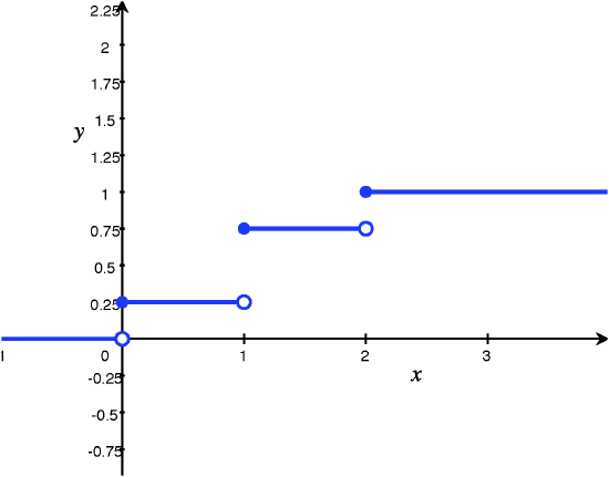
Figure 2: Graph of cdf in Example 3.2.4

Note that the cdf we found in Example 3.2.4 is a "step function", since its graph resembles a series of steps. This is the case for all discrete random variables. Additionally, the value of the cdf for a discrete random variable will always "jump" at the possible values of the random variable, and the size of the "jump" is given by the value of the pmf at that possible value of the random variable. For example, the graph in Figure 2 "jumps" from \(0.25\) to \(0.75\) at \(x=1\), so the size of the "jump" is \(0.75-0.25= 0.5\) and note that \(p(1) = P(X=1) = 0.5\). The pmf for any discrete random variable can be obtained from the cdf in this manner.

---

We end this section with a statement of the properties of cdf's.  The reader is encouraged to verify these properties hold for the cdf derived in Example 3.2.4 and to provide an intuitive explanation (or formal explanation using the axioms of probability and the properties of pmf's) for why these properties hold for cdf's in general.

Properties of Cumulative Distribution Functions

Let \(X\) be a random variable with cdf \(F\). Then \(F\) satisfies the following:

1. \(F\) is non-decreasing, i.e., \(F\) may be constant, but otherwise it is increasing.
2. \(\displaystyle{\lim_{x\to-\infty} F(x) = 0}\) and \(\displaystyle{\lim_{x\to\infty} F(x) = 1}\)