
9.3: Independent Samples for Two Means
- Page ID
- 16370

\( \newcommand{\vecs}[1]{\overset { \scriptstyle \rightharpoonup} {\mathbf{#1}} } \)
\( \newcommand{\vecd}[1]{\overset{-\!-\!\rightharpoonup}{\vphantom{a}\smash {#1}}} \)
\( \newcommand{\dsum}{\displaystyle\sum\limits} \)
\( \newcommand{\dint}{\displaystyle\int\limits} \)
\( \newcommand{\dlim}{\displaystyle\lim\limits} \)
\( \newcommand{\id}{\mathrm{id}}\) \( \newcommand{\Span}{\mathrm{span}}\)
( \newcommand{\kernel}{\mathrm{null}\,}\) \( \newcommand{\range}{\mathrm{range}\,}\)
\( \newcommand{\RealPart}{\mathrm{Re}}\) \( \newcommand{\ImaginaryPart}{\mathrm{Im}}\)
\( \newcommand{\Argument}{\mathrm{Arg}}\) \( \newcommand{\norm}[1]{\| #1 \|}\)
\( \newcommand{\inner}[2]{\langle #1, #2 \rangle}\)
\( \newcommand{\Span}{\mathrm{span}}\)
\( \newcommand{\id}{\mathrm{id}}\)
\( \newcommand{\Span}{\mathrm{span}}\)
\( \newcommand{\kernel}{\mathrm{null}\,}\)
\( \newcommand{\range}{\mathrm{range}\,}\)
\( \newcommand{\RealPart}{\mathrm{Re}}\)
\( \newcommand{\ImaginaryPart}{\mathrm{Im}}\)
\( \newcommand{\Argument}{\mathrm{Arg}}\)
\( \newcommand{\norm}[1]{\| #1 \|}\)
\( \newcommand{\inner}[2]{\langle #1, #2 \rangle}\)
\( \newcommand{\Span}{\mathrm{span}}\) \( \newcommand{\AA}{\unicode[.8,0]{x212B}}\)
\( \newcommand{\vectorA}[1]{\vec{#1}} % arrow\)
\( \newcommand{\vectorAt}[1]{\vec{\text{#1}}} % arrow\)
\( \newcommand{\vectorB}[1]{\overset { \scriptstyle \rightharpoonup} {\mathbf{#1}} } \)
\( \newcommand{\vectorC}[1]{\textbf{#1}} \)
\( \newcommand{\vectorD}[1]{\overrightarrow{#1}} \)
\( \newcommand{\vectorDt}[1]{\overrightarrow{\text{#1}}} \)
\( \newcommand{\vectE}[1]{\overset{-\!-\!\rightharpoonup}{\vphantom{a}\smash{\mathbf {#1}}}} \)
\( \newcommand{\vecs}[1]{\overset { \scriptstyle \rightharpoonup} {\mathbf{#1}} } \)
\(\newcommand{\longvect}{\overrightarrow}\)
\( \newcommand{\vecd}[1]{\overset{-\!-\!\rightharpoonup}{\vphantom{a}\smash {#1}}} \)
\(\newcommand{\avec}{\mathbf a}\) \(\newcommand{\bvec}{\mathbf b}\) \(\newcommand{\cvec}{\mathbf c}\) \(\newcommand{\dvec}{\mathbf d}\) \(\newcommand{\dtil}{\widetilde{\mathbf d}}\) \(\newcommand{\evec}{\mathbf e}\) \(\newcommand{\fvec}{\mathbf f}\) \(\newcommand{\nvec}{\mathbf n}\) \(\newcommand{\pvec}{\mathbf p}\) \(\newcommand{\qvec}{\mathbf q}\) \(\newcommand{\svec}{\mathbf s}\) \(\newcommand{\tvec}{\mathbf t}\) \(\newcommand{\uvec}{\mathbf u}\) \(\newcommand{\vvec}{\mathbf v}\) \(\newcommand{\wvec}{\mathbf w}\) \(\newcommand{\xvec}{\mathbf x}\) \(\newcommand{\yvec}{\mathbf y}\) \(\newcommand{\zvec}{\mathbf z}\) \(\newcommand{\rvec}{\mathbf r}\) \(\newcommand{\mvec}{\mathbf m}\) \(\newcommand{\zerovec}{\mathbf 0}\) \(\newcommand{\onevec}{\mathbf 1}\) \(\newcommand{\real}{\mathbb R}\) \(\newcommand{\twovec}[2]{\left[\begin{array}{r}#1 \\ #2 \end{array}\right]}\) \(\newcommand{\ctwovec}[2]{\left[\begin{array}{c}#1 \\ #2 \end{array}\right]}\) \(\newcommand{\threevec}[3]{\left[\begin{array}{r}#1 \\ #2 \\ #3 \end{array}\right]}\) \(\newcommand{\cthreevec}[3]{\left[\begin{array}{c}#1 \\ #2 \\ #3 \end{array}\right]}\) \(\newcommand{\fourvec}[4]{\left[\begin{array}{r}#1 \\ #2 \\ #3 \\ #4 \end{array}\right]}\) \(\newcommand{\cfourvec}[4]{\left[\begin{array}{c}#1 \\ #2 \\ #3 \\ #4 \end{array}\right]}\) \(\newcommand{\fivevec}[5]{\left[\begin{array}{r}#1 \\ #2 \\ #3 \\ #4 \\ #5 \\ \end{array}\right]}\) \(\newcommand{\cfivevec}[5]{\left[\begin{array}{c}#1 \\ #2 \\ #3 \\ #4 \\ #5 \\ \end{array}\right]}\) \(\newcommand{\mattwo}[4]{\left[\begin{array}{rr}#1 \amp #2 \\ #3 \amp #4 \\ \end{array}\right]}\) \(\newcommand{\laspan}[1]{\text{Span}\{#1\}}\) \(\newcommand{\bcal}{\cal B}\) \(\newcommand{\ccal}{\cal C}\) \(\newcommand{\scal}{\cal S}\) \(\newcommand{\wcal}{\cal W}\) \(\newcommand{\ecal}{\cal E}\) \(\newcommand{\coords}[2]{\left\{#1\right\}_{#2}}\) \(\newcommand{\gray}[1]{\color{gray}{#1}}\) \(\newcommand{\lgray}[1]{\color{lightgray}{#1}}\) \(\newcommand{\rank}{\operatorname{rank}}\) \(\newcommand{\row}{\text{Row}}\) \(\newcommand{\col}{\text{Col}}\) \(\renewcommand{\row}{\text{Row}}\) \(\newcommand{\nul}{\text{Nul}}\) \(\newcommand{\var}{\text{Var}}\) \(\newcommand{\corr}{\text{corr}}\) \(\newcommand{\len}[1]{\left|#1\right|}\) \(\newcommand{\bbar}{\overline{\bvec}}\) \(\newcommand{\bhat}{\widehat{\bvec}}\) \(\newcommand{\bperp}{\bvec^\perp}\) \(\newcommand{\xhat}{\widehat{\xvec}}\) \(\newcommand{\vhat}{\widehat{\vvec}}\) \(\newcommand{\uhat}{\widehat{\uvec}}\) \(\newcommand{\what}{\widehat{\wvec}}\) \(\newcommand{\Sighat}{\widehat{\Sigma}}\) \(\newcommand{\lt}{<}\) \(\newcommand{\gt}{>}\) \(\newcommand{\amp}{&}\) \(\definecolor{fillinmathshade}{gray}{0.9}\)This section will look at how to analyze when two samples are collected that are independent. As with all other hypothesis tests and confidence intervals, the process is the same though the formulas and assumptions are different. The only difference with the independent t-test, as opposed to the other tests that have been done, is that there are actually two different formulas to use depending on if a particular assumption is met or not.
Hypothesis Test for Independent t-Test (2-Sample t-Test)
- State the random variables and the parameters in words.
\(x_{1}\) = random variable 1
\(x_{2}\) = random variable 2
\(\mu_{1}\) = mean of random variable 1
\(\mu_{2}\)= mean of random variable 2 - State the null and alternative hypotheses and the level of significance The normal hypotheses would be
\(\begin{array}{ll}{H_{o} : \mu_{1}=\mu_{2}} & {\text { or } \quad H_{o} : \mu_{1}-\mu_{2}=0} \\ {H_{A} : \mu_{1}<\mu_{2}} & \quad\quad\: {H_{A} : \mu_{1}-\mu_{2}<0} \\ {H_{A} : \mu_{1}>\mu_{2}} & \quad\quad\: {H_{A} : \mu_{1}-\mu_{2}>0} \\ {H_{A} : \mu_{1} \neq \mu_{2}} & \quad\quad\: {H_{A} : \mu_{1}-\mu_{2} \neq 0}\end{array}\)
Also, state your \(\alpha\) level here. - State and check the assumptions for the hypothesis test
- A random sample of size \(n_{1}\) is taken from population 1. A random sample of size \(n_{2}\) is taken from population 2.
Note
The samples do not need to be the same size, but the test is more robust if they are.
- The two samples are independent.
- Population 1 is normally distributed. Population 2 is normally distributed. Just as before, the t-test is fairly robust to the assumption if the sample size is large. This means that if this assumption isn’t met, but your sample sizes are quite large (over 30), then the results of the t-test are valid.
- The population variances are unknown and not assumed to be equal. The old assumption is that the variances are equal. However, this assumption is no longer an assumption that most statisticians use. This is because it isn’t really realistic to assume that the variances are equal. So we will just assume the assumption of the variances being unknown and not assumed to be equal is true, and it will not be checked.
- A random sample of size \(n_{1}\) is taken from population 1. A random sample of size \(n_{2}\) is taken from population 2.
- Find the sample statistic, test statistic, and p-value
Sample Statistic:
Calculate \(\overline{x}_{1}, \overline{x}_{2}, s_{1}, s_{2}, n_{1}, n_{2}\)
Test Statistic:
Since the assumption that \(\sigma_{1}^{2}=\sigma_{2}^{2}\) isn’t being satisfied, then
\(t=\dfrac{\left(\overline{x}_{1}-\overline{x}_{2}\right)-\left(\mu_{1}-\mu_{2}\right)}{\sqrt{\stackrel{s_{1}^{2}}{n_{1}}+\stackrel{s_{2}^{2}}{n_{2}}}}\)
Usually \(\mu_{1}-\mu_{2}=0\), since \(H_{o} : \mu_{1}-\mu_{2}=0\)
Degrees of freedom: (the Welch–Satterthwaite equation)
\(d f=\dfrac{(A+B)^{2}}{\dfrac{A^{2}}{n_{1}-1}+\dfrac{B^{2}}{n_{2}-1}}\)
where \(A=\dfrac{s_{1}^{2}}{n_{1}} \text { and } B=\dfrac{s_{2}^{2}}{n_{2}}\)
p-value:
Using the TI-83/84: tcdf(lower limit, upper limit, df)Using R: pt(t, df)Note
If \(H_{A} : \mu_{1}-\mu_{2}<0\), then lower limit is \(-1 E 99\) and upper limit is your test statistic. If \(H_{A} : \mu_{1}-\mu_{2}>0\), then lower limit is your test statistic and the upper limit is \(1 E 99\). If \(H_{A} : \mu_{1}-\mu_{2} \neq 0\), then find the p-value for \(H_{A} : \mu_{1}-\mu_{2}<0\), and multiply by 2.
Note
If \(H_{A} : \mu_{1}-\mu_{2}<0\), then use pt(t, df). If \(H_{A} : \mu_{1}-\mu_{2}>0\), then use 1 - pt(t, df). If \(H_{A} : \mu_{1}-\mu_{2} \neq 0\), then find the p-value for \(H_{A} : \mu_{1}-\mu_{2}<0\), and multiply by 2.
- Conclusion
This is where you write reject \(H_{o}\) or fail to reject \(H_{o}\). The rule is: if the p-value < \(\alpha\), then reject \(H_{o}\). If the p-value \(\geq \alpha\), then fail to reject \(H_{o}\) - Interpretation This is where you interpret in real world terms the conclusion to the test. The conclusion for a hypothesis test is that you either have enough evidence to show \(H_{A}\) is true, or you do not have enough evidence to show \(H_{A}\) is true.
Confidence Interval for the Difference in Means from Two Independent Samples (2 Samp T-Int)
The confidence interval for the difference in means has the same random variables and means and the same assumptions as the hypothesis test for independent samples. If you have already completed the hypothesis test, then you do not need to state them again. If you haven’t completed the hypothesis test, then state the random variables and means and state and check the assumptions before completing the confidence interval step.
- Find the sample statistic and confidence interval
Sample Statistic:
Calculate Confidence Interval: \(\overline{x}_{1}, \overline{x}_{2}, s_{1}, s_{2}, n_{1}, n_{2}\)
The confidence interval estimate of the difference is \(\mu_{1}-\mu_{2}\)
Since the assumption that \(\sigma_{1}^{2}=\sigma_{2}^{2}\) isn’t being satisfied, then
\(\left(\overline{x}_{1}-\overline{x}_{2}\right)-E<\mu_{1}-\mu_{2}<\left(\overline{x}_{1}-\overline{x}_{2}\right)+E\)
where \(E=t_{c} \sqrt{\dfrac{s_{1}^{2}}{n_{1}}+\dfrac{s_{2}^{2}}{n_{2}}}\)
where \(t_{c}\) is the critical value with degrees of freedom:
Degrees of freedom: (the Welch–Satterthwaite equation)
\(d f=\dfrac{(A+B)^{2}}{\dfrac{A^{2}}{n_{1}-1}+\dfrac{B^{2}}{n_{2}-1}}\)
where \(A=\dfrac{s_{1}^{2}}{n_{1}} \text { and } B=\dfrac{s_{2}^{2}}{n_{2}}\) - Statistical Interpretation: In general this looks like, “there is a C% chance that \(\left(\overline{x}_{1}-\overline{x}_{2}\right)-E<\mu_{1}-\mu_{2}<\left(\overline{x}_{1}-\overline{x}_{2}\right)+E\) contains the true mean difference.”
- Real World Interpretation: This is where you state what interval contains the true difference in means, though often you state how much more (or less) the first mean is from the second mean.
The critical value is a value from the Student’s t-distribution. Since a confidence interval is found by adding and subtracting a margin of error amount from the difference in sample means, and the interval has a probability of containing the true difference in means, then you can think of this as the statement \(P\left(\left(\overline{x}_{1}-\overline{x}_{2}\right)-E<\mu_{1}-\mu_{2}<\left(\overline{x}_{1}-\overline{x}_{2}\right)+E\right)=C\). To find the critical value you use table A.2 in the Appendix.
How to check the assumptions of two sample t-test and confidence interval:
In order for the t-test or confidence interval to be valid, the assumptions of the test must be true. So whenever you run a t-test or confidence interval, you must make sure the assumptions are true. So you need to check them. Here is how you do this:
- For the random sample assumption, describe how you took the two samples. Make sure your sampling technique is random for both samples.
- For the independent assumption, describe how they are independent samples.
- For the assumption about each population being normally distributed, remember the process of assessing normality from chapter 6. Make sure you assess each sample separately.
- You do not need to check the equal variance assumption since it is not being assumed.
Example \(\PageIndex{1}\) hypothesis test for two means
The cholesterol level of patients who had heart attacks was measured two days after the heart attack. The researchers want to see if patients who have heart attacks have higher cholesterol levels over healthy people, so they also measured the cholesterol level of healthy adults who show no signs of heart disease. The data is in Table \(\PageIndex{1}\) ("Cholesterol levels after," 2013). Do the data show that people who have had heart attacks have higher cholesterol levels over patients that have not had heart attacks? Test at the 1% level.
| Cholesterol Level of Heart Attack Patients | Cholesterol Level of Healthy Individual |
|---|---|
| 270 | 196 |
| 236 | 232 |
| 210 | 200 |
| 142 | 242 |
| 280 | 206 |
| 272 | 178 |
| 160 | 184 |
| 220 | 198 |
| 226 | 160 |
| 242 | 182 |
| 186 | 182 |
| 266 | 198 |
| 206 | 182 |
| 318 | 238 |
| 294 | 198 |
| 282 | 188 |
| 234 | 166 |
| 224 | 204 |
| 276 | 182 |
| 282 | 178 |
| 360 | 212 |
| 310 | 164 |
| 280 | 230 |
| 278 | 186 |
| 288 | 162 |
| 288 | 182 |
| 244 | 218 |
| 236 | 170 |
| 200 | |
| 176 |
- State the random variables and the parameters in words.
- State the null and alternative hypotheses and the level of significance.
- State and check the assumptions for the hypothesis test.
- Find the sample statistic, test statistic, and p-value.
- Conclusion
- Interpretation
Solution
1. \(x_{1}\) = Cholesterol level of patients who had a heart attack
\(x_{2}\) = Cholesterol level of healthy individuals
\(\mu_{1}\) = mean cholesterol level of patients who had a heart attack
\(\mu_{2}\) = mean cholesterol level of healthy individuals
2. The normal hypotheses would be
\(\begin{array}{ll}{H_{o} : \mu_{1}=\mu_{2}} & {\text { or } \quad H_{o} : \mu_{1}-\mu_{2}=0} \\ {H_{A} : \mu_{1}>\mu_{2}} & \quad\quad\:{H_{A} : \mu_{1}-\mu_{2}>0} \\ {\alpha=0.01}\end{array}\)
3.
- A random sample of 28 cholesterol levels of patients who had a heart attack is taken. A random sample of 30 cholesterol levels of healthy individuals is taken. The problem does not state if either sample was randomly selected. So this assumption may not be valid.
- The two samples are independent. This is because either they were dealing with patients who had heart attacks or healthy individuals.
- Population of all cholesterol levels of patients who had a heart attack is normally distributed. Population of all cholesterol levels of healthy individuals is normally distributed.
Patients who had heart attacks:
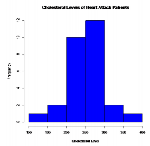.png?revision=1)
This looks somewhat bell shaped.
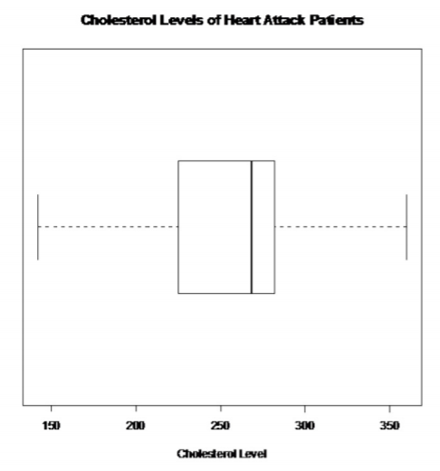.png?revision=1)
There are no outliers
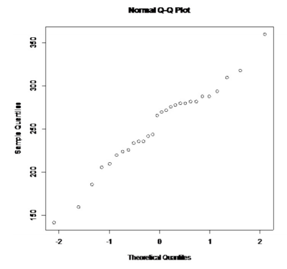.png?revision=1)
This looks somewhat linear.
So, the population of all cholesterol levels of patients who had heart attacks is probably somewhat normally distributed.
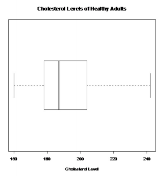
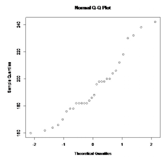
Healthy individuals:
.png?revision=1)
This does not look bell shaped.
.png?revision=1)
There are no outliers.
.png?revision=1)
This doesn't look linear.
So, the population of all cholesterol levels of healthy individuals is probably not normally distributed.
This assumption is not valid for the second sample. Since the sample is fairly large, and the t-test is robust, it may not be an issue. However, just realize that the conclusions of the test may not be valid.
4. Sample Statistic:
\(\overline{x}_{1} \approx 252.32, \overline{x}_{2} \approx 193.13, s_{1} \approx 47.0642, s_{2} \approx 22.3000, n_{1}=28, n_{2}=30\)
Test Statistic:
\(t=\dfrac{\left(\overline{x}_{1}-\overline{x}_{2}\right)-\left(\mu_{1}-\mu_{2}\right)}{\sqrt{\dfrac{s_{1}^{2}}{n_{1}}+\dfrac{s_{2}^{2}}{n_{2}}}}\)
\(=\dfrac{(252.32-193.13)-0}{\sqrt{\dfrac{47.0642^{2}}{28}+\dfrac{22.3000^{2}}{30}}}\)
\(\approx 6.051\)
Degrees of freedom: (the Welch-Satterthwaite equation)
\(A=\dfrac{s_{1}^{2}}{n_{1}}=\dfrac{47.0642^{2}}{28} \approx 79.1085\)
\(B=\dfrac{s_{2}^{2}}{n_{2}}=\dfrac{22.3000^{2}}{30} \approx 16.5763\)
\(d f=\dfrac{(A+B)^{2}}{\dfrac{A^{2}}{n_{1}-1}+\dfrac{B^{2}}{n_{2}-1}}=\dfrac{(79.1085+16.5763)^{2}}{\dfrac{79.1085^{2}}{28-1}+\dfrac{16.5763^{2}}{30-1}} \approx 37.9493\)
p-value:
Using TI-83/84: \(\operatorname{tcdf}(6.051,1 E 99,37.9493) \approx 2.44 \times 10^{-7}\)
Using R: \(1-\mathrm{pt}(6.051,37.9493) \approx 2.44 \times 10^{-7}\)
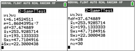
Using Technology: Using the TI-83/84:
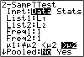.png?revision=1)
Note
The Pooled question on the calculator is for whether you are assuming the variances are equal. Since this assumption is not being made, then the answer to this question is no. Pooled means that you assume the variances are equal and can pool the sample variances together.
.png?revision=1)
Welch Two Sample t-test
data: heartattack and healthy
t = 6.1452, df = 37.675, p-value = 1.86e-07
alternative hypothesis: true difference in means is greater than 0
95 percent confidence interval:
44.1124 Inf
sample estimates:
mean of x mean of y
253.9286 193.1333
The test statistic is t = 6.1452. The p-value is \(1.86 \times 10^{-7}\)
5. Reject \(H_{o}\) since the p-value < \(\alpha\).
6. This is enough evidence to show that patients who have had heart attacks have higher cholesterol level on average from healthy individuals. (Though do realize that some of assumptions are not valid, so this interpretation may be invalid.)
Example \(\PageIndex{2}\) confidence interval for \(\mu_{1}-\mu_{2}\)
The cholesterol level of patients who had heart attacks was measured two days after the heart attack. The researchers want to see if patients who have heart attacks have higher cholesterol levels over healthy people, so they also measured the cholesterol level of healthy adults who show no signs of heart disease. The data is in Example \(\PageIndex{1}\) ("Cholesterol levels after," 2013). Find a 99% confidence interval for the mean difference in cholesterol levels between heart attack patients and healthy individuals.
- State the random variables and the parameters in words.
- State and check the assumptions for the hypothesis test.
- Find the sample statistic and confidence interval.
- Statistical Interpretation
- Real World Interpretation
Solution
1. These were stated in Example \(\PageIndex{1}\), but are reproduced here for reference.
\(x_{1}\) = Cholesterol level of patients who had a heart attack
\(x_{2}\) = Cholesterol level of healthy individuals
\(\mu_{1}\) = mean cholesterol level of patients who had a heart attack
\(\mu_{2}\) = mean cholesterol level of healthy individuals
2. The assumptions were stated and checked in Example \(\PageIndex{1}\).
3. Sample Statistic:
\(\overline{x}_{1} \approx 252.32, \overline{x_{2}} \approx 193.13, s_{1} \approx 47.0642, s_{2} \approx 22.3000, n_{1}=28, n_{2}=30\)
Test Statistic:
Degrees of freedom: (the Welch–Satterthwaite equation)
\(A=\dfrac{s_{1}^{2}}{n_{1}}=\dfrac{47.0642^{2}}{28} \approx 79.1085\)
\(B=\dfrac{s_{2}^{2}}{n_{2}}=\dfrac{22.3000^{2}}{30} \approx 16.5763\)
\(d f=\dfrac{(A+B)^{2}}{\dfrac{A^{2}}{n_{1}-1}+\dfrac{B^{2}}{n_{2}-1}}=\dfrac{(79.1085+16.5763)^{2}}{\dfrac{79.1085^{2}}{28-1}+\dfrac{16.5763^{2}}{30-1}} \approx 37.9493\)
Since this df is not in the table, round to the nearest whole number.
\(t_{c}=2.712\)
\(E=t_{c} \sqrt{\dfrac{s_{1}^{2}}{n_{1}}+\dfrac{s_{2}^{2}}{n_{2}}}=2.712 \sqrt{\dfrac{47.0642^{2}}{28}+\dfrac{22.3000^{2}}{30}} \approx 26.53\)
\(\left(\overline{x}_{1}-\overline{x}_{2}\right)-E<\mu_{1}-\mu_{2}<\left(\overline{x}_{1}-\overline{x}_{2}\right)+E\)
\((252.32-193.13)-26.53<\mu_{1}-\mu_{2}<(252.32-193.13)+26.53\)
\(32.66 \mathrm{mg} / \mathrm{dL}<\mu_{1}-\mu_{2}<85.72 \mathrm{mg} / \mathrm{dL}\)
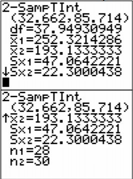
Using Technology:
Using TI-83/84:
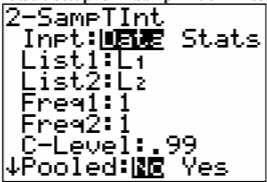.png?revision=1)
Note
The Pooled question on the calculator is for whether you are assuming the variances are equal. Since this assumption is not being made, then the answer to this question is no. Pooled means that you assume the variances are equal and can pool the sample variances together.
.png?revision=1)
Using R: the commands is t.test(variable1, variable2, conf.level=C), where C is in decimal form.
For this example, the command is
t.test(heartattack, healthy, conf.level=.99)
Output:
Welch Two Sample t-test
data: heartattack and healthy
t = 6.1452, df = 37.675, p-value = 3.721e-07
alternative hypothesis: true difference in means is not equal to 0
99 percent confidence interval:
33.95750 87.63298
sample estimates:
mean of x mean of y
253.9286 193.1333
The confidence interval is \(33.96<\mu_{1}-\mu_{2}<87.63\)
4. There is a 99% chance that \(33.96<\mu_{1}-\mu_{2}<87.63\) contains the true difference in means.
5. The mean cholesterol level for patients who had heart attacks is anywhere from 32.66 mg/dL to 85,72 mg/dL more than the mean cholesterol level for healthy patients. (Though do realize that many of assumptions are not valid, so this interpretation may be invalid.)
If you do assume that the variances are equal, that is \(\sigma_{1}^{2}=\sigma_{2}^{2}\), then the test statistic is:
\(t=\dfrac{\left(\overline{x}_{1}-\overline{x}_{2}\right)-\left(\mu_{1}-\mu_{2}\right)}{s_{p} \sqrt{\dfrac{1}{n_{1}}+\dfrac{1}{n_{2}}}}\)
where \(s_{p}=\sqrt{\dfrac{\left(n_{1}-1\right) s_{1}^{2}+\left(n_{2}-1\right) s_{2}^{2}}{\left(n_{1}-1\right)+\left(n_{2}-1\right)}}\)
\(s_{p}\) = pooled standard deviation
The Degrees of Freedom is: df = \(n_{1}+n_{2}-2\)
The confidence interval if you do assume that \(\sigma_{1}^{2}=\sigma_{2}^{2}\) has been met, is
\(\left(\overline{x}_{1}-\overline{x}_{2}\right)-E<\mu_{1}-\mu_{2}<\left(\overline{x}_{1}-\overline{x}_{2}\right)+E\)
where \(E=t_{c} s_{p} \sqrt{\dfrac{1}{n_{1}}+\dfrac{1}{n_{2}}}\)
and \(s_{p}=\sqrt{\dfrac{\left(n_{1}-1\right) s_{1}^{2}+\left(n_{2}-1\right) s_{2}^{2}}{\left(n_{1}-1\right)+\left(n_{2}-1\right)}}\)
Degrees of Freedom: df = \(n_{1}+n_{2}-2\)
\(t_{c}\) is the critical value where C = 1 - \(\alpha\)
To show that the variances are equal, just show that the ratio of your sample variances is not unusual (probability is greater than 0.05). In other words, make sure the following is true.
\(P\left(F>s_{1}^{2} / s_{2}^{2}\right) \geq 0.05\left(\text { or } P\left(F>s_{2}^{2} / s_{1}^{2}\right) \geq 0.05\right.\) so that the larger variance is in the numerator). This probability is from an F-distribution. To find the probability on the TI-83/84 calculator use \(\operatorname{Fcdf}\left(s_{1}^{2} / s_{2}^{2}, 1 E 99, n_{1}-1, n_{2}-1\right)\). To find the probability on R, use \(1-\operatorname{pf}\left(s_{1}^{2} / s_{2}^{2}, n_{1}-1, n_{2}-1\right)\).
Note
The F-distribution is very sensitive to the normal distribution. A better test for equal variances is Levene's test, though it is more complicated. It is best to do Levene’s test when using statistical software (such as SPSS or Minitab) to perform the two-sample independent t-test.
Example \(\PageIndex{3}\) hypothesis test for two means
The amount of sodium in beef hotdogs was measured. In addition, the amount of sodium in poultry hotdogs was also measured ("SOCR 012708 id," 2013). The data is in Example \(\PageIndex{2}\). Is there enough evidence to show that beef has less sodium on average than poultry hotdogs? Use a 5% level of significance.
| Sodium in Beef Hotdogs | Sodium in Poultry Hotdogs |
|---|---|
| 495 | 430 |
| 477 | 375 |
| 425 | 396 |
| 322 | 383 |
| 482 | 387 |
| 587 | 542 |
| 370 | 359 |
| 322 | 357 |
| 479 | 528 |
| 375 | 513 |
| 330 | 426 |
| 300 | 513 |
| 386 | 358 |
| 401 | 581 |
| 645 | 588 |
| 440 | 522 |
| 317 | 545 |
| 319 | 430 |
| 298 | 375 |
| 253 | 396 |
- State the random variables and the parameters in words.
- State the null and alternative hypotheses and the level of significance.
- State and check the assumptions for the hypothesis test.
- Find the sample statistic, test statistic, and p-value.
- Conclusion
- Interpretation
Solution
1. \(x_{1}\) = sodium level in beef hotdogs
\(x_{2}\) = sodium level in poultry hotdogs
\(\mu_{1}\) = mean sodium level in beef hotdogs
\(\mu_{2}\) = mean sodium level in poultry hotdogs
2. The normal hypotheses would be
\(\begin{array}{ll}{H_{o} : \mu_{1}=\mu_{2}} & {\text { or } \quad H_{o} : \mu_{1}-\mu_{2}=0} \\ {H_{A} : \mu_{1}<\mu_{2}} & \quad\quad\: {H_{A} : \mu_{1}-\mu_{2}<0} \\ {\alpha=0.05}\end{array}\)
3.
- A random sample of 20 sodium levels in beef hotdogs is taken. A random sample of 20 sodium levels in poultry hotdogs. The problem does not state if either sample was randomly selected. So this assumption may not be valid.
- The two samples are independent since these are different types of hotdogs.
- Population of all sodium levels in beef hotdogs is normally distributed. Population of all sodium levels in poultry hotdogs is normally distributed. Beef Hotdogs:
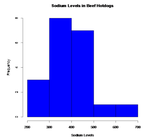.png?revision=1)
This looks somewhat bell shaped.
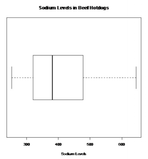.png?revision=1)
There are no outliers.
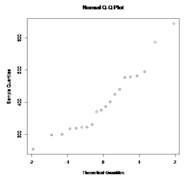.png?revision=1)
This looks somewhat linear.
So, the population of all sodium levels in beef hotdogs may be normally distributed.
Poultry Hotdogs:
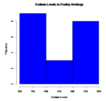.png?revision=1)
This does not look bell shaped.
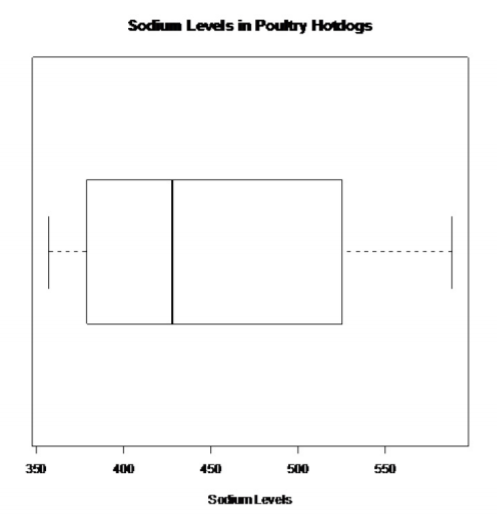.png?revision=1)
There are no outliers.
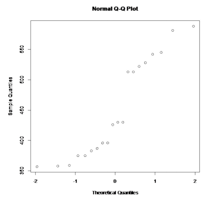.png?revision=1)
This does not look linear.
So, the population of all sodium levels in poultry hotdogs is probably not normally distributed.
This assumption is not valid. Since the samples are fairly large, and the t-test is robust, it may not be a large issue. However, just realize that the conclusions of the test may not be valid.
d. The population variances are equal, i.e. \(\sigma_{1}^{2}=\sigma_{2}^{2}\).
\(\begin{array}{l}{s_{1} \approx 102.4347} \\ {s_{2} \approx 81.1786} \\ {\dfrac{s_{1}^{2}}{s_{2}^{2}}=\dfrac{102.4347^{2}}{81.1786^{2}} \approx 1.592}\end{array}\)
Using TI-83/84: Fcdf \((1.592,1 E 99,19,19) \approx 0.1597 \geq 0.05\)
Using R: 1 - pf \((1.592,19,19) \approx 0.1597 \geq 0.05\)
So you can say that these variances are equal.
4. Find the sample statistic, test statistic, and p-value
Sample Statistic:
\(\overline{x}_{1}=401.15, \overline{x}_{2}=450.2, s_{1} \approx 102.4347, s_{2} \approx 81.1786, n_{1}=20, n_{2}=20\)
Test Statistic:
The assumption \(\sigma_{1}^{2}=\sigma_{2}^{2}\) has been met, so
\(s_{p}=\sqrt{\dfrac{\left(n_{1}-1\right) s_{1}^{2}+\left(n_{2}-1\right) s_{2}^{2}}{\left(n_{1}-1\right)+\left(n_{2}-1\right)}}\)
\(=\sqrt{\dfrac{102.4347^{2} * 19+81.1786^{2} * 19}{(20-1)+(20-1)}}\)
\(\approx 92.4198\)
Though you should try to do the calculations in the problem so you don’t create round off error.
\(t=\dfrac{\left(\overline{x}_{1}-\overline{x}_{2}\right)-\left(\mu_{1}-\mu_{2}\right)}{s_{P} \sqrt{\dfrac{1}{n_{1}}+\dfrac{1}{n_{2}}}}\)
\(=\dfrac{(401.15-450.2)-0}{92.4198 \sqrt{\dfrac{1}{20}+\dfrac{1}{20}}}\)
\(\approx-1.678\)
df = 20 + 20 - 2 = 38
p-value:
Using TI-83/84: tcdf \((-1 E 99,-1.678,38) \approx 0.0508\)
Using R: pt \((-1.678,38) \approx 0.0508\)
Using technology to find the t and p-value:
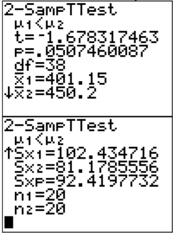
Using TI-83/84:
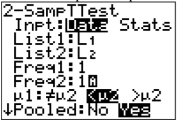.png?revision=1)
Note
The Pooled question on the calculator is for whether you are using the pooled standard deviation or not. In this example, the pooled standard deviation was used since you are assuming the variances are equal. That is why the answer to the question is Yes.
.png?revision=1)
Using R: the command is t.test(variable1, variable2, alternative="less" or "greater")
For this example, the command is
t.test(beef, poultry, alternative="less", equalvar=TRUE)
Welch Two Sample t-test
data: beef and poultry
t = -1.6783, df = 36.115, p-value = 0.05096
alternative hypothesis: true difference in means is less than 0
95 percent confidence interval:
-Inf 0.2875363
sample estimates:
mean of x mean of y
401.15 450.20
The t = -1.6783 and the p-value = 0.05096.
5. Fail to reject \(H_{o}\) since the p-value > \(\alpha\).
6. This is not enough evidence to show that beef hotdogs have less sodium than poultry hotdogs. (Though do realize that many of assumptions are not valid, so this interpretation may be invalid.)
Example \(\PageIndex{4}\) confidence interval for \(\mu_{1}-\mu_{2}\)
The amount of sodium in beef hotdogs was measured. In addition, the amount of sodium in poultry hotdogs was also measured ("SOCR 012708 id," 2013). The data is in Example \(\PageIndex{2}\). Find a 95% confidence interval for the mean difference in sodium levels between beef and poultry hotdogs.
- State the random variables and the parameters in words.
- State and check the assumptions for the hypothesis test.
- Find the sample statistic and confidence interval.
- Statistical Interpretation
- Real World Interpretation
Solution
1. These were stated in Example \(\PageIndex{1}\), but are reproduced here for reference.
\(x_{1}\) = sodium level in beef hotdogs
\(x_{2}\) = sodium level in poultry hotdogs
\(\mu_{1}\) = mean sodium level in beef hotdogs
\(\mu_{2}\) = mean sodium level in poultry hotdogs
2. The assumptions were stated and checked in Example \(\PageIndex{3}\).
3. Sample Statistic:
\(\overline{x}_{1}=401.15, \overline{x}_{2}=450.2, s_{1} \approx 102.4347, s_{2} \approx 81.1786, n_{1}=20, n_{2}=20\)
Confidence Interval:
The confidence interval estimate of the difference \(\mu_{1}-\mu_{2}\) is
The assumption \(\sigma_{1}^{2}=\sigma_{2}^{2}\) has been met, so
\(s_{p}=\sqrt{\dfrac{\left(n_{1}-1\right) s_{1}^{2}+\left(n_{2}-1\right) s_{2}^{2}}{\left(n_{1}-1\right)+\left(n_{2}-1\right)}}\)
\(=\sqrt{\dfrac{102.4347^{2} * 19+81.1786^{2} * 19}{(20-1)+(20-1)}}\)
\(\approx 92.4198\)
Though you should try to do the calculations in the formula for E so you don’t create round off error.
df = \(=n_{1}+n_{2}-2=20+20-2=38\)
\(t_{c} = 2.024\)
\(E=t_{c} s_{p} \sqrt{\dfrac{1}{n_{1}}+\dfrac{1}{n_{2}}}\)
\(=2.024(92.4198) \sqrt{\dfrac{1}{20}+\dfrac{1}{20}}\)
\(\approx 59.15\)
\(\left(\overline{x}_{1}-\overline{x}_{2}\right)-E<\mu_{1}-\mu_{2}<\left(\overline{x}_{1}-\overline{x}_{2}\right)+E\)
\((401.15-450.2)-59.15<\mu_{1}-\mu_{2}<(401.15-450.2)+59.15\)
\(-108.20 \mathrm{g}<\mu_{1}-\mu_{2}<10.10 \mathrm{g}\)
Using technology:
Using the TI-83/84:
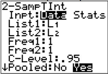.png?revision=1)
Note
The Pooled question on the calculator is for whether you are using the pooled standard deviation or not. In this example, the pooled standard deviation was used since you are assuming the variances are equal. That is why the answer to the question is Yes.
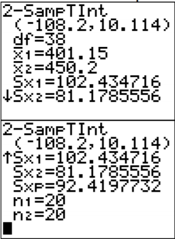.png?revision=1)
Using R: the command is t.test(variable1, variable2, equalvar=TRUE, conf.level=C), where C is in decimal form.
For this example, the command is
t.test(beef, poultry, conf.level=.95, equalvar=TRUE)
Welch Two Sample t-test
data: beef and poultry
t = -1.6783, df = 36.115, p-value = 0.1019
alternative hypothesis: true difference in means is not equal to 0
95 percent confidence interval:
-108.31592 10.21592
sample estimates:
mean of x mean of y
401.15 450.20
The confidence interval is \(-108.32<\mu_{1}-\mu_{2}<10.22\).
4. There is a 95% chance that \(-108.20 \mathrm{g}<\mu_{1}-\mu_{2}<10.10 \mathrm{g}\) contains the true difference in means.
5. The mean sodium level of beef hotdogs is anywhere from 108.20 g less than the mean sodium level of poultry hotdogs to 10.10 g more. (The negative sign on the lower limit implies that the first mean is less than the second mean. The positive sign on the upper limit implies that the first mean is greater than the second mean.)
Realize that many of assumptions are not valid in this example, so the interpretation may be invalid.
Homework
Exercise \(\PageIndex{1}\)
In each problem show all steps of the hypothesis test or confidence interval. If some of the assumptions are not met, note that the results of the test or interval may not be correct and then continue the process of the hypothesis test or confidence interval. Unless directed by your instructor, do not assume the variances are equal (except in problems 11 through 16).
- The income of males in each state of the United States, including the District of Columbia and Puerto Rico, are given in Example \(\PageIndex{3}\), and the income of females is given in table #9.3.4 ("Median income of," 2013). Is there enough evidence to show that the mean income of males is more than of females? Test at the 1% level.
$42,951 $52,379 $42,544 $37,488 $49,281 $50,987 $60,705 $50,411 $66,760 $40,951 $43,902 $45,494 $41,528 $50,746 $45,183 $43,624 $43,993 $41,612 $46,313 $43,944 $56,708 $60,264 $50,053 $50,580 $40,202 $43,146 $41,635 $42,182 $41,803 $53,033 $60,568 $41,037 $50,388 $41,950 $44,660 $46,176 $41,420 $45,976 $47,956 $22,529 $48,842 $41,464 $40,285 $41,309 $43,160 $47,573 $44,057 $52,805 $53,046 $42,125 $46,214 $51,630 Table \(\PageIndex{3}\): Data of Income for Males $31,862 $40,550 $36,048 $30,752 $41,817 $40,236 $47,476 $40,500 $60,332 $33,823 $35,438 $37,242 $31,238 $39,150 $34,023 $33,745 $33,269 $32,684 $31,844 $34,599 $48,748 $46,185 $36,931 $40,416 $29,548 $33,865 $31,067 $33,424 $35,484 $41,021 $47,155 $32,316 $42,113 $33,459 $32,462 $35,746 $31,274 $36,027 $37,089 $22,117 $41,412 $31,330 $31,329 $33,184 $35,301 $32,843 $38,177 $40,969 $40,993 $29,688 $35,890 $34,381 Table \(\PageIndex{4}\): Data of Income for Females - The income of males in each state of the United States, including the District of Columbia and Puerto Rico, are given in Example \(\PageIndex{3}\), and the income of females is given in Example \(\PageIndex{4}\) ("Median income of," 2013). Compute a 99% confidence interval for the difference in incomes between males and females in the U.S.
- A study was conducted that measured the total brain volume (TBV) (in \(m m^{3}\)) of patients that had schizophrenia and patients that are considered normal. Example \(\PageIndex{5}\) contains the TBV of the normal patients and Example \(\PageIndex{6}\) contains the TBV of schizophrenia patients ("SOCR data oct2009," 2013). Is there enough evidence to show that the patients with schizophrenia have less TBV on average than a patient that is considered normal? Test at the 10% level.
1663407 1583940 1299470 1535137 1431890 1578698 1453510 1650348 1288971 1366346 1326402 1503005 1474790 1317156 1441045 1463498 1650207 1523045 1441636 1432033 1420416 1480171 1360810 1410213 1574808 1502702 1203344 1319737 1688990 1292641 1512571 1635918 Table \(\PageIndex{5}\): Total Brain Volume (in \(\mathrm{mm}^{3}\)) of Normal Patients 1331777 1487886 1066075 1297327 1499983 1861991 1368378 1476891 1443775 1337827 1658258 1588132 1690182 1569413 1177002 1387893 1483763 1688950 1563593 1317885 1420249 1363859 1238979 1286638 1325525 1588573 1476254 1648209 1354054 1354649 1636119 Table \(\PageIndex{6}\): Total Brain Volume (in \(\mathrm{mm}^{3}\)) of Schizophrenia Patients - A study was conducted that measured the total brain volume (TBV) (in \(m m^{3}\)) of patients that had schizophrenia and patients that are considered normal. Example \(\PageIndex{5}\) contains the TBV of the normal patients and Example \(\PageIndex{6}\) contains the TBV of schizophrenia patients ("SOCR data oct2009," 2013). Compute a 90% confidence interval for the difference in TBV of normal patients and patients with Schizophrenia.
- The length of New Zealand (NZ) rivers that travel to the Pacific Ocean are given in Example \(\PageIndex{7}\) and the lengths of NZ rivers that travel to the Tasman Sea are given in Example \(\PageIndex{8}\) ("Length of NZ," 2013). Do the data provide enough evidence to show on average that the rivers that travel to the Pacific Ocean are longer than the rivers that travel to the Tasman Sea? Use a 5% level of significance.
209 48 169 138 64 97 161 95 145 90 121 80 56 64 209 64 72 288 322 Table \(\PageIndex{7}\): Lengths (in km) of NZ Rivers that Flow into the Pacific Ocean 76 64 68 64 37 32 32 51 56 40 64 56 80 121 177 56 80 35 72 72 108 48 Table \(\PageIndex{8}\): Lengths (in km) of NZ Rivers that Flow into the Tasman Sea - The length of New Zealand (NZ) rivers that travel to the Pacific Ocean are given in Example \(\PageIndex{7}\) and the lengths of NZ rivers that travel to the Tasman Sea are given in Example \(\PageIndex{8}\) ("Length of NZ," 2013). Estimate the difference in mean lengths of rivers between rivers in NZ that travel to the Pacific Ocean and ones that travel to the Tasman Sea. Use a 95% confidence level.
- The number of cell phones per 100 residents in countries in Europe is given in Example \(\PageIndex{9}\) for the year 2010. The number of cell phones per 100 residents in countries of the Americas is given in Example \(\PageIndex{10}\) also for the year 2010 ("Population reference bureau," 2013). Is there enough evidence to show that the mean number of cell phones in countries of Europe is more than in countries of the Americas? Test at the 1% level.
100 76 100 130 75 84 112 84 138 133 118 134 126 188 129 93 64 128 124 122 109 121 127 152 96 63 99 95 151 147 123 95 67 67 118 125 110 115 140 115 141 77 98 102 102 112 118 118 54 23 121 126 47 Table \(\PageIndex{9}\): Number of Cell Phones per 100 Residents in Europe 158 117 106 159 53 50 78 66 88 92 42 3 150 72 86 113 50 58 70 109 37 32 85 101 75 69 55 115 95 73 86 157 100 119 81 113 87 105 96 Table \(\PageIndex{10}\): Number of Cell Phones per 100 Residents in the America - The number of cell phones per 100 residents in countries in Europe is given in Example \(\PageIndex{9}\) for the year 2010. The number of cell phones per 100 residents in countries of the Americas is given in Example \(\PageIndex{10}\) also for the year 2010 ("Population reference bureau," 2013). Find the 98% confidence interval for the difference in mean number of cell phones per 100 residents in Europe and the Americas.
- A vitamin K shot is given to infants soon after birth. Nurses at Northbay Healthcare were involved in a study to see if how they handle the infants could reduce the pain the infants feel ("SOCR data nips," 2013). One of the measurements taken was how long, in seconds, the infant cried after being given the shot. A random sample was taken from the group that was given the shot using conventional methods (Example \(\PageIndex{11}\)), and a random sample was taken from the group that was given the shot where the mother held the infant prior to and during the shot (Example \(\PageIndex{12}\)). Is there enough evidence to show that infants cried less on average when they are held by their mothers than if held using conventional methods? Test at the 5% level.
63 0 2 46 33 33 29 23 11 12 48 15 33 14 51 37 24 70 63 0 73 39 54 52 39 34 30 55 58 18 Table \(\PageIndex{11}\): Crying Time of Infants Given Shots Using Conventional Methods 0 32 20 23 14 19 60 59 64 64 72 50 44 14 10 58 19 41 17 5 36 73 19 46 9 43 73 27 25 18 Table \(\PageIndex{12}\): Crying Time of Infants Given Shots Using New Methods - A vitamin K shot is given to infants soon after birth. Nurses at Northbay Healthcare were involved in a study to see if how they handle the infants could reduce the pain the infants feel ("SOCR data nips," 2013). One of the measurements taken was how long, in seconds, the infant cried after being given the shot. A random sample was taken from the group that was given the shot using conventional methods (Example \(\PageIndex{11}\)), and a random sample was taken from the group that was given the shot where the mother held the infant prior to and during the shot (Example \(\PageIndex{12}\)). Calculate a 95% confidence interval for the mean difference in mean crying time after being given a vitamin K shot between infants held using conventional methods and infants held by their mothers.
- Redo problem 1 testing for the assumption of equal variances and then use the formula that utilizes the assumption of equal variances (follow the procedure in Example \(\PageIndex{3}\)).
- Redo problem 2 testing for the assumption of equal variances and then use the formula that utilizes the assumption of equal variances (follow the procedure in Example \(\PageIndex{3}\)).
- Redo problem 7 testing for the assumption of equal variances and then use the formula that utilizes the assumption of equal variances (follow the procedure in Example \(\PageIndex{3}\)).
- Redo problem 8 testing for the assumption of equal variances and then use the formula that utilizes the assumption of equal variances (follow the procedure in Example \(\PageIndex{3}\)).
- Redo problem 9 testing for the assumption of equal variances and then use the formula that utilizes the assumption of equal variances (follow the procedure in Example \(\PageIndex{3}\)).
- Redo problem 10 testing for the assumption of equal variances and then use the formula that utilizes the assumption of equal variances (follow the procedure in Example \(\PageIndex{3}\)).
- Answer
-
For all hypothesis tests, just the conclusion is given. For all confidence intervals, just the interval using technology is given. See solution for the entire answer.
- Reject Ho
- \(\$ 65443.80<\mu_{1}-\mu_{2}<\$ 13340.80\)
- Fail to reject Ho
- \(-51564.6 \mathrm{mm}^{3}<\mu_{1}-\mu_{2}<75656.6 \mathrm{mm}^{3}\)
- Reject Ho
- \(23.2818 \mathrm{km}<\mu_{1}-\mu_{2}<103.67 \mathrm{km}\)
- Reject Ho
- \(4.3641<\mu_{1}-\mu_{2}<37.5276\)
- Fail to reject Ho
- \(-10.9726 \mathrm{s}<\mu_{1}-\mu_{2}<11.3059 \mathrm{s}\)
- Reject Ho
- \(\$ 6544.98<\mu_{1}-\mu_{2}<\$ 13339.60\)
- Reject Ho
- \(4.8267<\mu_{1}-\mu_{2}<37.0649\)
- Fail to reject Ho
- \(-10.9713 \mathrm{s}<\mu_{1}-\mu_{2}<11.3047 \mathrm{s}\)