3.1: The Least Squares Regression Line

Suppose we have some bivariate quantitative data {(x₁, y₁), . . . , (x_n, y_n)} for which the correlation coefficient indicates some linear association. It is natural to want to write down explicitly the equation of the best line through the data – the question is what is this line. The most common meaning given to best in this search for the line is the line whose total square error is the smallest possible. We make this notion precise in two steps

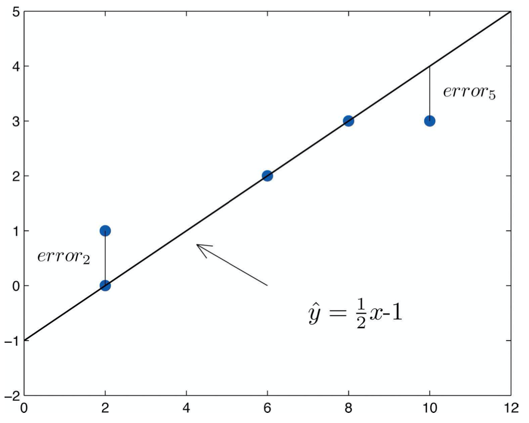
DEFINITION 3.1.1. Given a bivariate quantitative dataset {(x₁, y₁), . . . , (x_n, y_n)} and a candidate line \(\ \hat{y} = mx+b\) passing through this dataset, a residual is the difference in y-coordinates of an actual data point (x_i, y_i) and the line’s y value at the same x-coordinate. That is, if the y-coordinate of the line when x = x_i is \(\ \hat{y_i} = mx_i + b\), then the residual is the measure of error given by \(\ error_i = y_i - \hat{y_i}\).

Note we use the convention here and elsewhere of writing \(\ \hat{y}\) for the y-coordinate on an approximating line, while the plain y variable is left for actual data values, like y_i.

Here is an example of what residuals look like

Now we are in the position to state the

DEFINITION 3.1.2. Given a bivariate quantitative dataset the least square regression line, almost always abbreviated to LSRL, is the line for which the sum of the squares of the residuals is the smallest possible.

FACT 3.1.3. If a bivariate quantitative dataset {(x₁, y₁), . . . , (x_n, y_n)} has LSRL given \(\ \hat{y} = mx + b\), then

1. The slope of the LSRL is given by \(\ m=r\frac{s_y}{s_x}\), where r is the correlation coefficient of the dataset.
2. The LSRL passes through the point (\(\ \bar{x},\bar{y}\)).
3. It follows that the y-intercept of the LSRL is given by \(\ b = \bar{y} - \bar{x}m = \bar{y} - \bar{x}r \frac{s_y}{s_x}\)

It is possible to find the (coefficients of the) LSRL using the above information, but it is often more convenient to use a calculator or other electronic tool. Such tools also make it very easy to graph the LSRL right on top of the scatterplot – although it is often fairly easy to sketch what the LSRL will likely look like by just making a good guess, using visual intuition, if the linear association is strong (as will be indicated by the correlation coefficient).

EXAMPLE 3.1.4. Here is some data where the individuals are 23 students in a statistics class, the independent variable is the students’ total score on their homeworks, while the dependent variable is their final total course points, both out of 100.

\(\begin{array}{llllllllll}{x:} & {65} & {65} & {50} & {53} & {59} & {92} & {86} & {84} & {29}\end{array}\)
\(\begin{array}{rrrrrrrrrr}{y:} & {74} & {71} & {65} & {60} & {83} & {90} & {84} & {88} & {48}\end{array}\)

\(\begin{array}{lllllllllll}{x:} & {29} & {09} & {64} & {31} & {69} & {10} & {57} & {81} & {81}\end{array}\)
\(\begin{array}{lllllllllll}{y:} & {54} & {25} & {79} & {58} & {81} & {29} & {81} & {94} & {86}\end{array}\)

\(\begin{array}{lllllllllll}{x:} & {80} & {70} & {60} & {62} & {59} \end{array}\)
\(\begin{array}{lllllllllll}{y:} & {95} & {68} & {69} & {83} & {70} \end{array}\)

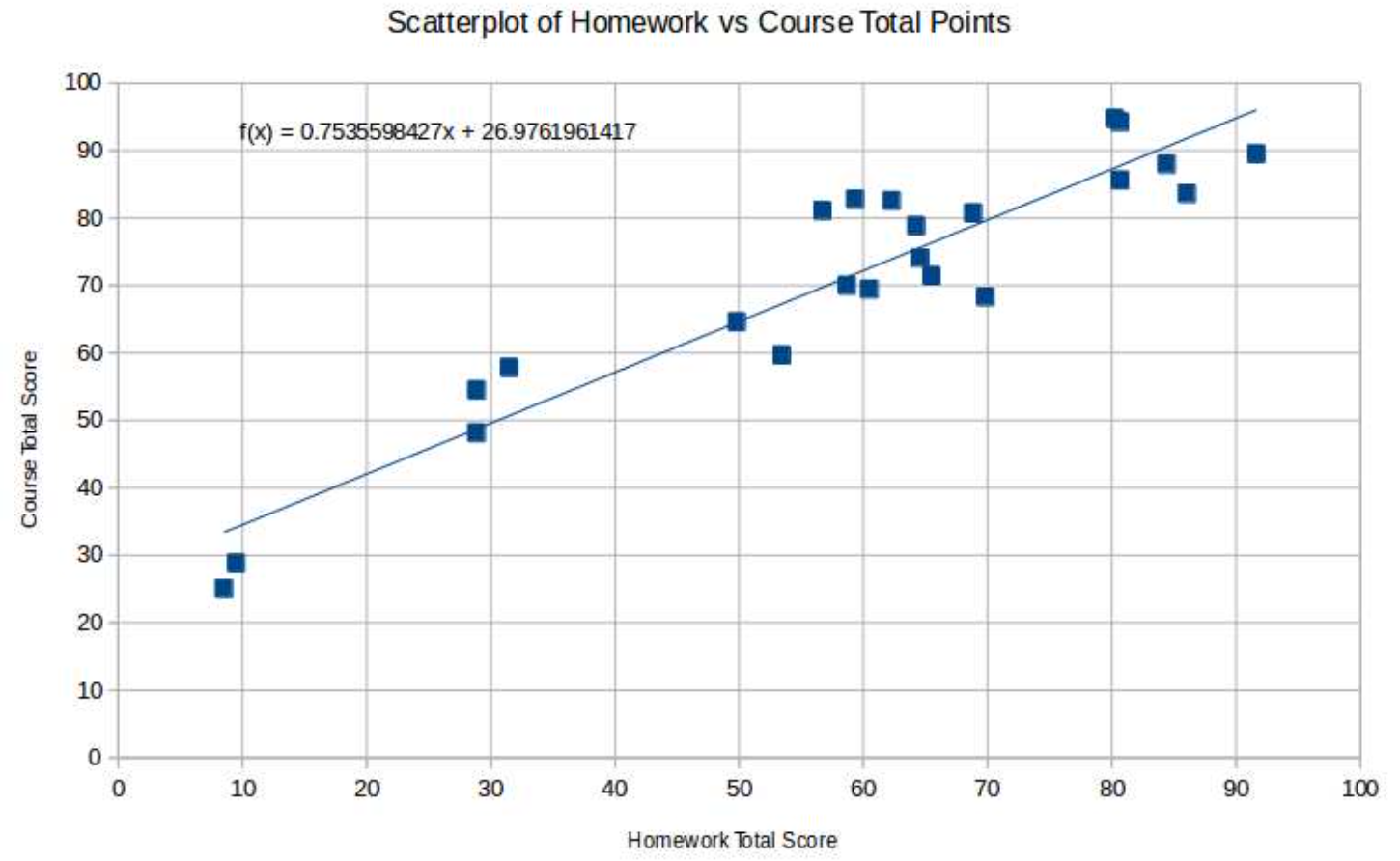
Here is the resulting scatterplot, made with LibreOffice Calc(a free equivalent of Mi- crosoft Excel)

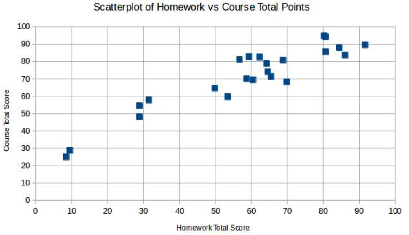
It seems pretty clear that there is quite a strong linear association between these two vari- ables, as is born out by the correlation coefficient, r = .935 (computed with LibreOffice Calc’s CORREL). Using then STDEV.S and AVERAGE, we find that the coefficients of the LSRL for this data, \(\ \hat{y} = mx + b\) are

\(\ m = r \frac{s_y}{s_x} = .935 \frac{18.701}{23.207} = .754\) and \(\ b = \bar{y} - \bar{x}m =71 − 58 · .754 = 26.976\)

We can also use LibreOffice Calc’s Insert Trend Line, with Show Equation, to get all this done automatically. Note that when LibreOffice Calc writes the equation of the LSRL, it uses f (x) in place of \(\ \hat{y}\), as we would.