12.1: Testing a Single Mean
- Page ID
- 2152
Learning Objectives
- Compute the probability of a sample mean being at least as high as a specified value when \(\sigma\) is known
- Compute a two-tailed probability
- Compute the probability of a sample mean being at least as high as a specified value when \(\sigma\) is estimated
- State the assumptions required for item \(3\) above
This section shows how to test the null hypothesis that the population mean is equal to some hypothesized value. For example, suppose an experimenter wanted to know if people are influenced by a subliminal message and performed the following experiment. Each of nine subjects is presented with a series of \(100\) pairs of pictures. As a pair of pictures is presented, a subliminal message is presented suggesting the picture that the subject should choose. The question is whether the (population) mean number of times the suggested picture is chosen is equal to \(50\). In other words, the null hypothesis is that the population mean (\(\mu\)) is \(50\). The (hypothetical) data are shown in Table \(\PageIndex{1}\). The data in Table \(\PageIndex{1}\) have a sample mean (\(M\)) of \(51\). Thus the sample mean differs from the hypothesized population mean by \(1\).
| Frequency |
|---|
| 45 |
| 48 |
| 49 |
| 49 |
| 51 |
| 52 |
| 53 |
| 55 |
| 57 |
The significance test consists of computing the probability of a sample mean differing from \(\mu\) by one (the difference between the hypothesized population mean and the sample mean) or more. The first step is to determine the sampling distribution of the mean. As shown in a previous section, the mean and standard deviation of the sampling distribution of the mean are
\[μ_M = μ\]
and
\[\sigma_M = \dfrac{\sigma}{\sqrt{N}}\]
respectively. It is clear that \(\mu _M=50\). In order to compute the standard deviation of the sampling distribution of the mean, we have to know the population standard deviation (\(\sigma\)).
The current example was constructed to be one of the few instances in which the standard deviation is known. In practice, it is very unlikely that you would know \(\sigma\) and therefore you would use \(s\), the sample estimate of \(\sigma\). However, it is instructive to see how the probability is computed if \(\sigma\) is known before proceeding to see how it is calculated when \(\sigma\) is estimated.
For the current example, if the null hypothesis is true, then based on the binomial distribution, one can compute that variance of the number correct is
\[\sigma ^2 = N\pi (1-\pi ) = 100(0.5)(1-0.5) = 25\]
Therefore, \(\sigma =5\). For a \(\sigma \) of \(5\) and an \(N\) of \(9\), the standard deviation of the sampling distribution of the mean is \(5/3 = 1.667\). Recall that the standard deviation of a sampling distribution is called the standard error.
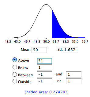
To recap, we wish to know the probability of obtaining a sample mean of \(51\) or more when the sampling distribution of the mean has a mean of \(50\) and a standard deviation of \(1.667\). To compute this probability, we will make the assumption that the sampling distribution of the mean is normally distributed. We can then use the normal distribution calculator as shown in Figure \(\PageIndex{1}\).

Notice that the mean is set to \(50\), the standard deviation to \(1.667\), and the area above \(51\) is requested and shown to be \(0.274\).
Therefore, the probability of obtaining a sample mean of \(51\) or larger is \(0.274\). Since a mean of \(51\) or higher is not unlikely under the assumption that the subliminal message has no effect, the effect is not significant and the null hypothesis is not rejected.
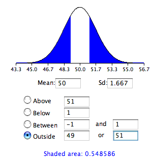
The test conducted above was a one-tailed test because it computed the probability of a sample mean being one or more points higher than the hypothesized mean of \(50\) and the area computed was the area above \(51\). To test the two-tailed hypothesis, you would compute the probability of a sample mean differing by one or more in either direction from the hypothesized mean of \(50\). You would do so by computing the probability of a mean being less than or equal to \(49\) or greater than or equal to \(51\).
The results of the normal distribution calculator are shown in Figure \(\PageIndex{2}\).

As you can see, the probability is \(0.548\) which, as expected, is twice the probability of \(0.274\) shown in Figure \(\PageIndex{1}\).
Before normal calculators such as the one illustrated above were widely available, probability calculations were made based on the standard normal distribution. This was done by computing \(Z\) based on the formula
\[Z=\frac{M-\mu }{\sigma _M}\]
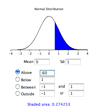
where \(Z\) is the value on the standard normal distribution, \(M\) is the sample mean, \(\mu\) is the hypothesized value of the mean, and \(\sigma _M\) is the standard error of the mean. For this example, \(Z = (51-50)/1.667 = 0.60\). Use the normal calculator, with a mean of \(0\) and a standard deviation of \(1\), as shown below.

Notice that the probability (the shaded area) is the same as previously calculated (for the one-tailed test).
As noted, in real-world data analysis it is very rare that you would know \(\sigma\) and wish to estimate \(\mu\). Typically \(\sigma\) is not known and is estimated in a sample by \(s\), and \(\sigma _M\) is estimated by \(s_M\).
Example \(\PageIndex{1}\): adhd treatment
Consider the data in the "ADHD Treatment" case study. These data consist of the scores of \(24\) children with ADHD on a delay of gratification (DOG) task. Each child was tested under four dosage levels. Table \(\PageIndex{2}\) shows the data for the placebo (\(0\) mg) and highest dosage level (\(0.6\) mg) of methylphenidate. Of particular interest here is the column labeled "Diff" that shows the difference in performance between the \(0.6\) mg (\(D60\)) and the \(0\) mg (\(D0\)) conditions. These difference scores are positive for children who performed better in the \(0.6\) mg condition than in the control condition and negative for those who scored better in the control condition. If methylphenidate has a positive effect, then the mean difference score in the population will be positive. The null hypothesis is that the mean difference score in the population is \(0\).
Table \(\PageIndex{2}\): DOG scores as a function of dosage
| D0 | D60 | Diff |
|---|---|---|
| 57 | 62 | 5 |
| 27 | 49 | 22 |
| 32 | 30 | -2 |
| 31 | 34 | 3 |
| 34 | 38 | 4 |
| 38 | 36 | -2 |
| 71 | 77 | 6 |
| 33 | 51 | 18 |
| 34 | 45 | 11 |
| 53 | 42 | -11 |
| 36 | 43 | 7 |
| 42 | 57 | 15 |
| 26 | 36 | 10 |
| 52 | 58 | 6 |
| 36 | 35 | -1 |
| 55 | 60 | 5 |
| 36 | 33 | -3 |
| 42 | 49 | 7 |
| 36 | 33 | -3 |
| 54 | 59 | 5 |
| 34 | 35 | 1 |
| 29 | 37 | 8 |
| 33 | 45 | 12 |
| 33 | 29 | -4 |
Solution
To test this null hypothesis, we compute \(t\) using a special case of the following formula:
\[t=\frac{\text{statistic-hypothesized value}}{\text{estimated standard error of the statistic}}\]
The special case of this formula applicable to testing a single mean is
\[t=\frac{M-\mu }{s_M}\]
where \(t\) is the value we compute for the significance test, \(M\) is the sample mean, \(\mu\) is the hypothesized value of the population mean, and \(s_M\) is the estimated standard error of the mean. Notice the similarity of this formula to the formula for Z.
In the previous example, we assumed that the scores were normally distributed. In this case, it is the population of difference scores that we assume to be normally distributed.
The mean (\(M\)) of the \(N = 24\) difference scores is \(4.958\), the hypothesized value of \(\mu\) is \(0\), and the standard deviation (\(s\)) is \(7.538\). The estimate of the standard error of the mean is computed as:
\[s_M=\frac{s}{\sqrt{N}}=\frac{7.5382}{\sqrt{24}}=1.54\]
Therefore,
\[t =\frac{4.96}{1.54} = 3.22\]
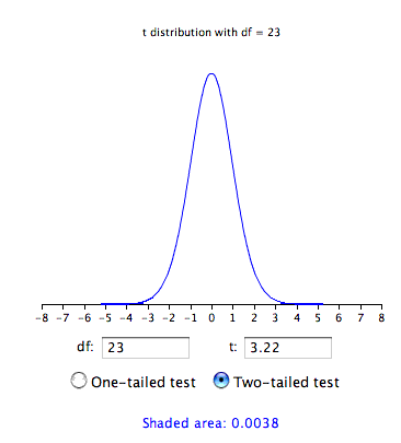
The probability value for \(t\) depends on the degrees of freedom. The number of degrees of freedom is equal to \(N - 1 = 23\). As shown below, the t distribution calculator finds that the probability of a \(t\) less than \(-3.22\) or greater than \(3.22\) is only \(0.0038\). Therefore, if the drug had no effect, the probability of finding a difference between means as large or larger (in either direction) than the difference found is very low. Therefore the null hypothesis that the population mean difference score is zero can be rejected. The conclusion is that the population mean for the drug condition is higher than the population mean for the placebo condition.

Review of Assumptions
- Each value is sampled independently from each other value.
- The values are sampled from a normal distribution.


