1.2: Stationary Time Series

Fitting solely independent and identically distributed random variables to data is too narrow a concept. While, on one hand, they allow for a somewhat nice and easy mathematical treatment, their use is, on the other hand, often hard to justify in applications. Our goal is therefore to introduce a concept that keeps some of the desirable properties of independent and identically distributed random variables ("regularity''), but that also considerably enlarges the class of stochastic processes to choose from by allowing dependence as well as varying distributions. Dependence between two random variables \(X\) and \(Y\) is usually measured in terms of the \(covariance\) \(function\)

\[ Cov(X,Y)=E\big[(X-E[X])(Y-E[Y])\big] \nonumber \]

and the \(correlation\) \(function\)

\[ Corr(X,Y)=\frac{Cov(X,Y)}{\sqrt{Var(X)Var(Y)}}. \nonumber \]

With these notations at hand, the classes of strictly and weakly dependent stochastic processes can be introduced.

Definition 1.2.1 (Strict Stationarity). A stochastic process (\(X_t\colon t\in T\)) is called strictly stationary if, for all \(t_1,...,t_n \in T\) and \(h\) such that \(t_1+h,...,t_n+h\in T\), it holds that
\[ (
X_{t_1},\ldots,X_{t_n})
\stackrel{\cal D}{=}
(X_{t_1+h},\ldots,X_{t_n+h}).
\nonumber \]
That is, the so-called finite-dimensional distributions of the process are invariant under time shifts. Here \(=^{\cal D}\) indicates equality in distribution.

The definition in terms of the finite-dimensional distribution can be reformulated equivalently in terms of the cumulative joint distribution function equalities

\[ P(X_{t_1}\leq x_1,\ldots,X_{t_n}\leq x_n)=P(X_{t_1+h}\leq x_1,\ldots,X_{t_n+h}\leq x_n) \nonumber \]

holding true for all \(x_1,...,x_n\in\mathbb{R}\), \(t_1,...,t_n\in T\) and \(h\) such that \(t_1+h,...,t_n+h\in T\). This can be quite difficult to check for a given time series, especially if the generating mechanism of a time series is far from simple, since too many model parameters have to be estimated from the available data, rendering concise statistical statements impossible. A possible exception is provided by the case of independent and identically distributed random variables.

To get around these difficulties, a time series analyst will commonly only specify the first- and second-order moments of the joint distributions. Doing so then leads to the notion of weak stationarity.

Definition 1.2.2 (Weak Stationarity). A stochastic process \((X_t\colon t\in T)\) is called weakly stationary if

• the second moments are finite: \(E[X_t^2]<\infty\) for all \(t\in T\);
• the means are constant: \(E[X_t]=m\) for all \(t\in T\);
• the covariance of \(X_t\) and \(X_{t+h}\) depends on \(h\) only:

\[ \gamma(h)=\gamma_X(h)=Cov(X_t,X_{t+h}), \qquad h\in T \mbox{ such that } t+h\in T, \nonumber \]
is independent of \(t\in T\) and is called the autocovariance function (ACVF). Moreover,
\[ \rho(h)=\rho_X(h)=\frac{\gamma(h)}{\gamma(0)},\qquad h\in T, \nonumber \]
is called the autocorrelation function (ACF).

Remark 1.2.1. If \((X_t: t\in T)\)) is a strictly stationary stochastic process with finite second moments, then it is also weakly stationary. The converse is not necessarily true. If \((X_t\colon t\in T)\), however, is weakly stationary and Gaussian, then it is also strictly stationary. Recall that a stochastic process is called Gaussian if, for any \(t_1,...,t_n\in T\), the random vector \((X_{t_1},...,X_{t_n})\) is multivariate normally distributed.

This section is concluded with examples of stationary and nonstationary stochastic processes.

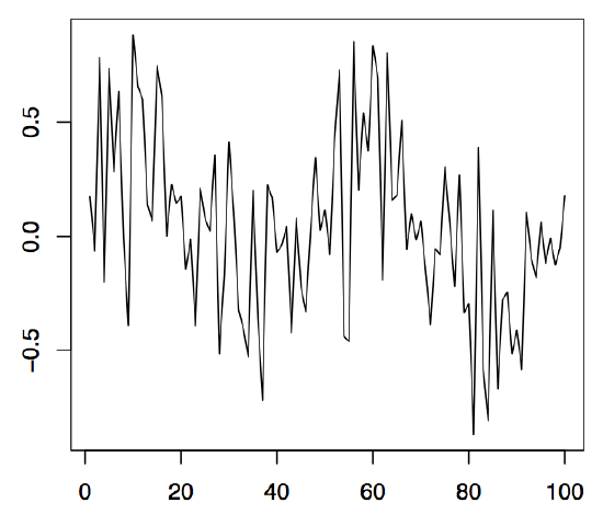
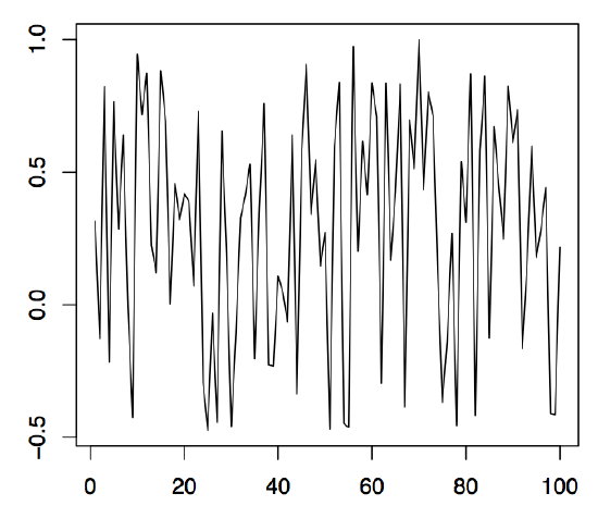
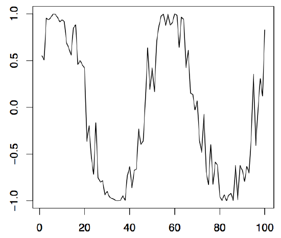
• Figure 1.5: 100 simulated values of the cyclical time series (left panel), the stochastic amplitude (middle panel), and the sine part (right panel).

Example 1.2.1 (White Noise). Let \((Z_t\colon t\in\mathbb{Z})\) be a sequence of real-valued, pairwise uncorrelated random variables with \(E[Z_t]=0\) and \(0<Var(Z_t)=\sigma^2<\infty\) for all \(t\in\mathbb{Z}\). Then \((Z_t\colon t\in Z)\) is called white noise, abbreviated by \((Z_t\colon t\in\mathbb{Z})\sim{\rm WN}(0,\sigma^2)\). It defines a centered, weakly stationary process with ACVF and ACF given by
\[
\gamma(h)=\left\{\begin{array}{r@{\quad\;}l} \sigma^2, & h=0, \\ 0, & h\not=0,\end{array}\right.
\qquad\mbox{and}\qquad
\rho(h)=\left\{\begin{array}{r@{\quad\;}l} 1, & h=0, \\ 0, & h\not=0,\end{array}\right.
\nonumber \]
respectively. If the \((Z_t\colon t\in\mathbb{Z})\) are moreover independent and identically distributed, they are called iid noise, shortly \((Z_t\colon t\in\mathbb{Z})\sim{\rm IID}(0,\sigma^2)\). The left panel of Figure 1.6 displays 1000 observations of an iid noise sequence \((Z_t\colon t\in\mathbb{Z})\) based on standard normal random variables. The corresponding R commands to produce the plot are

> z = rnorm(1000,0,1)
> plot.ts(z, xlab="", ylab="", main="")

The command rnorm simulates here 1000 normal random variables with mean 0 and variance 1. There are various built-in random variable generators in R such as the functions runif(n,a,b) and rbinom(n,m,p) which simulate the \(n\) values of a uniform distribution on the interval \((a,b)\) and a binomial distribution with repetition parameter \(m\) and success probability \(p\), respectively.

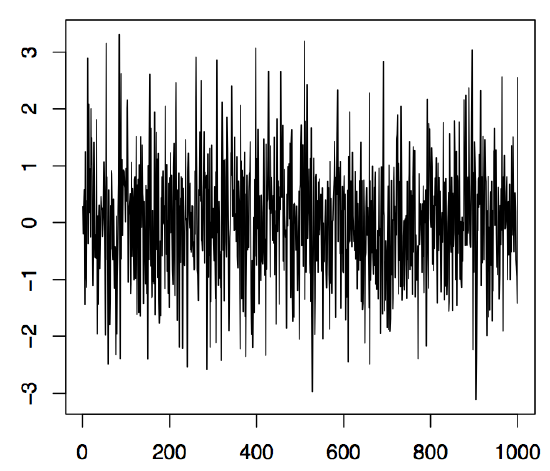
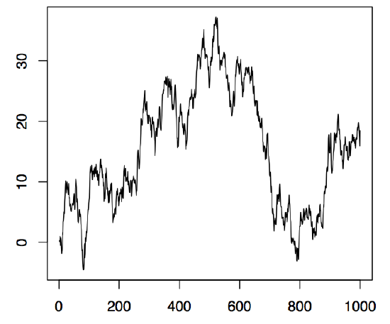
Figure 1.6: 1000 simulated values of iid N(0, 1) noise (left panel) and a random walk with iid N(0, 1) innovations (right panel).

Example 1.2.2 (Cyclical Time Series). Let \(A\) and \(B\) be uncorrelated random variables with zero mean and variances \(Var(A)=Var(B)=\sigma^2\), and let \(\lambda\in\mathbb{R}\) be a frequency parameter. Define
\[
X_t=A\cos(\lambda t)+B\sin(\lambda t),\qquad t\in\mathbb{R}.
\nonumber \]
The resulting stochastic process \((X_t\colon t\in\mathbb{R})\) is then weakly stationary. Since \(\sin(\lambda t+\varphi)=\sin(\varphi)\cos(\lambda t)+\cos(\varphi)\sin(\lambda t)\), the process can be represented as
\[
X_t=R\sin(\lambda t+\varphi), \qquad t\in\mathbb{R},
\nonumber \]
so that \(R\) is the stochastic amplitude and \(\varphi\in[-\pi,\pi]\) the stochastic phase of a sinusoid. Some computations show that one must have \(A=R\sin(\varphi)\) and \(B=R\cos(\varphi)\). In the left panel of Figure 1.5, 100 observed values of a series \((X_t)_{t\in \mathbb{Z}}\) are displayed. Therein, \(\lambda=\pi/25\) was used, while \(R\) and \(\varphi\) were random variables uniformly distributed on the interval \((-.5,1)\) and \((0,1)\), respectively. The middle panel shows the realization of \(R\), the right panel the realization of \(\sin(\lambda t+\varphi)\). Using cyclical time series bears great advantages when seasonal effects, such as annually recurrent phenomena, have to be modeled. The following R commands can be applied:

> t = 1:100; R = runif(100,-.5,1); phi = runif(100,0,1); lambda = pi/25
> cyc = R*sin(lambda*t+phi)
> plot.ts(cyc, xlab="", ylab="")

This produces the left panel of Figure 1.5. The middle and right panels follow in a similar fashion.

Example 1.2.3 (Random Walk). Let \((Z_t\colon t\in\mathbb{N})\sim{\rm WN}(0,\sigma^2)\). Let \(S_0=0\) and
\[
S_t=Z_1+\ldots+Z_t,\qquad t\in\mathbb{N}.
\nonumber \]
The resulting stochastic process \((S_t\colon t\in\mathbb{N}_0)\) is called a random walk and is the most important nonstationary time series. Indeed, it holds here that, for \(h>0\),
\[
Cov(S_t,S_{t+h})=Cov(S_t,S_t+R_{t,h})=t\sigma^2,
\nonumber \]
where \(R_{t,h}=Z_{t+1}+\ldots+Z_{t+h}\), and the ACVF obviously depends on \(t\). In R, one may construct a random walk, for example, with the following simple command that utilizes the 1000 normal observations stored in the array z of Example 1.2.1.

> rw = cumsum(z)
The function cumsum takes as input an array and returns as output an array of the same length that contains as its jth entry the sum of the first j input entries. The resulting time series plot is shown in the right panel of Figure 1.6.

Chapter 3 discusses in detail so-called autoregressive moving average processes which have become a central building block in time series analysis. They are constructed from white noise sequences by an application of a set of stochastic difference equations similar to the ones defining the random walk \((S_t\colon t\in\mathbb{N}_0)\) of Example 1.2.3.

In general, the true parameters of a stationary stochastic process \((X_t\colon t\in T)\) are unknown to the statistician. Therefore, they have to be estimated from a realization \(x_1,...,x_n\). The following set of estimators will be used here. The sample mean of \(x_1,...,x_n\) is defined as
\[
\bar{x}=\frac 1n\sum_{t=1}^nx_t.
\nonumber \]
The sample autocovariance function (sample ACVF) is given by
\begin{equation}\label{eq:1.2.1}
\hat{\gamma}(h)=
\frac 1n\sum_{t=1}^{n-h}(x_{t+h}-\bar{x})(x_t-\bar{x}),
\qquad h=0,1,\ldots,n-1.
\end{equation}
Finally, the sample autocorrelation function (sample ACF) is
\[
\hat{\rho}(h)=\frac{\hat{\gamma}(h)}{\hat{\gamma}(0)},
\qquad h=0,1,\ldots,n-1.
\nonumber \]

Example 1.2.4. Let \((Z_t\colon t\in\mathbb{Z})\) be a sequence of independent standard normally distributed random variables (see the left panel of Figure 1.6 for a typical realization of size n = 1,000). Then, clearly, \(\gamma(0)=\rho(0)=1\) and \(\gamma(h)=\rho(h)=0\) whenever \(h\not=0\). Table 1.1 gives the corresponding estimated values \(\hat{\gamma}(h)\) and \(\hat{\rho}(h)\) for \(h=0,1,\ldots,5\).

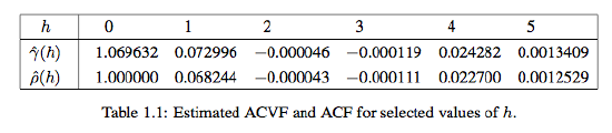
The estimated values are all very close to the true ones, indicating that the estimators work reasonably well for n = 1,000. Indeed it can be shown that they are asymptotically unbiased and consistent. Moreover, the sample autocorrelations \(\hat{\rho}(h)\) are approximately normal with zero mean and variance \(1/1000\). See also Theorem 1.2.1 below. In R, the function acf can be used to compute the sample ACF.

Theorem 1.2.1. Let \((Z_t\colon t\in\mathbb{Z})\sim{\rm WN}(0,\sigma^2)\) and let \(h\not=0\). Under a general set of conditions, it holds that the sample ACF at lag \(h\), \(\hat{\rho}(h)\), is for large \(n\) approximately normally distributed with zero mean and variance 1/n.

Theorem 1.2.1 and Example 1.2.4 suggest a first method to assess whether or not a given data set can be modeled conveniently by a white noise sequence: for a white noise sequence, approximately 95% of the sample ACFs should be within the the confidence interval \(\pm2/\sqrt{n}\). Using the data files on the course webpage, one can compute with R the corresponding sample ACFs to check for whiteness of the underlying time series. The properties of the sample ACF are revisited in Chapter 2.

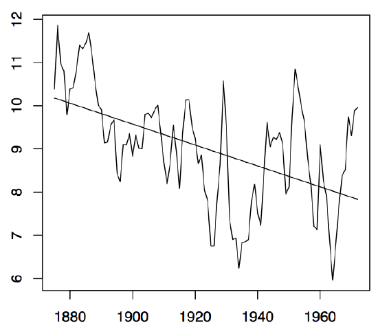
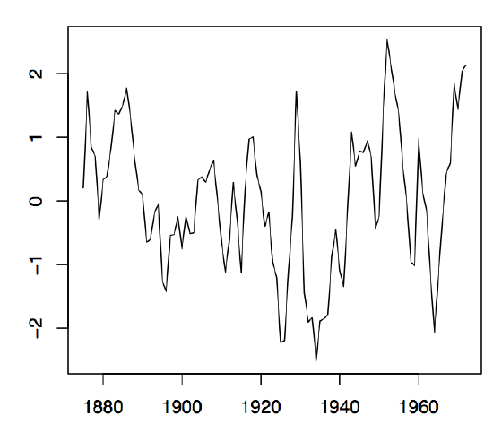
• Figure1.7: Annual water levels of Lake Huron (left panel) and the residual plot obtained from fitting a linear trend to the data (right panel).