
5.5: Comparing many Means with ANOVA (Special Topic)
- Page ID
- 296

Sometimes we want to compare means across many groups. We might initially think to do pairwise comparisons; for example, if there were three groups, we might be tempted to compare the first mean with the second, then with the third, and then finally compare the second and third means for a total of three comparisons. However, this strategy can be treacherous. If we have many groups and do many comparisons, it is likely that we will eventually nd a difference just by chance, even if there is no difference in the populations.
In this section, we will learn a new method called analysis of variance (ANOVA) and a new test statistic called F. ANOVA uses a single hypothesis test to check whether the means across many groups are equal:
- H0: The mean outcome is the same across all groups. In statistical notation, \(\mu _1 = \mu _2 = \dots = \mu _k\) where \(\mu _i\) represents the mean of the outcome for observations in category i.
- HA: At least one mean is different.
Generally we must check three conditions on the data before performing ANOVA:
- the observations are independent within and across groups,
- the data within each group are nearly normal, and
- the variability across the groups is about equal.
When these three conditions are met, we may perform an ANOVA to determine whether the data provide strong evidence against the null hypothesis that all the \(\mu _i\) are equal.
Example \(\PageIndex{1}\)
College departments commonly run multiple lectures of the same introductory course each semester because of high demand. Consider a statistics department that runs three lectures of an introductory statistics course. We might like to determine whether there are statistically significant differences infirstexam scores in these three classes (A, B, and C). Describe appropriate hypotheses to determine whether there are any differences between the three classes.
Solution
The hypotheses may be written in the following form:
- H0: The average score is identical in all lectures. Any observed difference is due to chance. Notationally, we write \(\mu _A = \mu _B = \mu _C\).
- HA: The average score varies by class. We would reject the null hypothesis in favor of the alternative hypothesis if there were larger differences among the class averages than what we might expect from chance alone.
Strong evidence favoring the alternative hypothesis in ANOVA is described by unusually large differences among the group means. We will soon learn that assessing the variability of the group means relative to the variability among individual observations within each group is key to ANOVA's success.
Example \(\PageIndex{2}\)
Examine Figure \(\PageIndex{1}\). Compare groups I, II, and III. Can you visually determine if the differences in the group centers is due to chance or not? Now compare groups IV, V, and VI. Do these differences appear to be due to chance?
Figure \(\PageIndex{1}\): Side-by-side dot plot for the outcomes for six groups.
Solution
Any real difference in the means of groups I, II, and III is difficult to discern, because the data within each group are very volatile relative to any differences in the average outcome. On the other hand, it appears there are differences in the centers of groups IV, V, and VI. For instance, group V appears to have a higher mean than that of the other two groups. Investigating groups IV, V, and VI, we see the differences in the groups' centers are noticeable because those differences are large relative to the variability in the individual observations within each group.
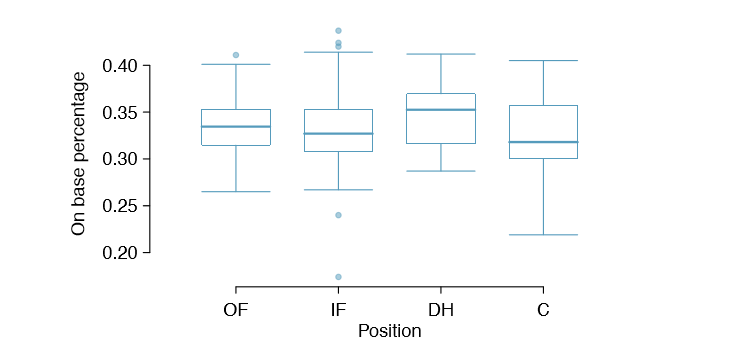
Is Batting Performance Related to Player Position in MLB?
We would like to discern whether there are real differences between the batting performance of baseball players according to their position: out elder (OF), in elder (IF), designated hitter (DH), and catcher (C). We will use a data set called bat10, which includes batting records of 327 Major League Baseball (MLB) players from the 2010 season. Six of the 327 cases represented in bat10 are shown in Table \(\PageIndex{1}\), and descriptions for each variable are provided in Table 5.26. The measure we will use for the player batting performance (the outcome variable) is on-base percentage (OBP). The on-base percentage roughly represents the fraction of the time a player successfully gets on base or hits a home run.
| name | team | position | AB | H | HR | RBI | AVG | OBP | |
|---|---|---|---|---|---|---|---|---|---|
| 1 | I Suzuki | SEA | OF | 680 | 214 | 6 | 43 | 0.315 | 0.359 |
| 2 | D Jeter | NYY | IF | 663 | 179 | 10 | 67 | 0.270 | 0.340 |
| 3 | M Young | TEX | IF | 656 | 186 | 21 | 91 | 0.284 | 0.330 |
| \(\vdots\) | \(\vdots\) | \(\vdots\) | \(\vdots\) | \(\vdots\) | \(\vdots\) | \(\vdots\) | \(\vdots\) | \(\vdots\) | \(\vdots\) |
| 325 | B Molina | SF | C | 202 | 52 | 3 | 17 | 0.257 | 0.312 |
| 326 | J Thole | NTM | C | 202 | 56 | 3 | 17 | 0.277 | 0.357 |
| 327 | C Heisey | CIN | OF | 201 | 51 | 8 | 21 | 0.254 | 0.324 |
Exercise \(\PageIndex{1}\)
The null hypothesis under consideration is the following: \[\mu _{OF} = \mu _{IF} = \mu _{DH} = \mu _{C}. \]Write the null and corresponding alternative hypotheses in plain language.
Solution
- H0: The average on-base percentage is equal across the four positions.
- HA: The average on-base
| variable |
description |
|---|---|
| name | Player name |
| team | The abbreviated name of the player's team |
| position | The player's primary eld position (OF, IF, DH, C) |
| AB | Number of opportunities at bat |
| H | Number of hits |
| HR | Number of home runs |
| RBI | Number of runs batted in |
| AVG | Batting average, which is equal to H=AB |
| OBP | On-base percentage, which is roughly equal to the fraction of times a player gets on base or hits a home run |
Example \(\PageIndex{3}\)
The player positions have been divided into four groups: outfield (OF), infield (IF), designated hitter (DH), and catcher (C). What would be an appropriate point estimate of the batting average by out elders, \(\mu _{OF}\)?
Solution
A good estimate of the batting average by out elders would be the sample average of AVG for just those players whose position is out field:
\[\bar {x}_{OF} = 0.334.\]
Table \(\PageIndex{3}\) provides summary statistics for each group. A side-by-side box plot for the batting average is shown in Figure \(\PageIndex{1}\). Notice that the variability appears to be approximately constant across groups; nearly constant variance across groups is an important assumption that must be satisfied before we consider the ANOVA approach.
| OF | IF | DH | C | |
|---|---|---|---|---|
| Sample size (\(n_i\)) | 120 | 154 | 14 | 39 |
| Sample mean (\(\bar {x}_i\)) | 0.334 | 0.332 | 0.348 | 0.323 |
| Sample SD (\(s_i\)) | 0.029 | 0.037 | 0.036 | 0.045 |
percentage varies across some (or all) groups.
Example \(\PageIndex{1}\)
The largest difference between the sample means is between the designated hitter and the catcher positions. Consider again the original hypotheses:
- H0: \(\mu _{OF} = \mu _{IF} = \mu _{DH} = \mu _{C}\)
- HA: The average on-base percentage (\(\mu _i\)) varies across some (or all) groups.
Why might it be inappropriate to run the test by simply estimating whether the difference of \(\mu _{DH}\) and \(\mu _{C}\) is statistically significant at a 0.05 significance level?
Solution
The primary issue here is that we are inspecting the data before picking the groups that will be compared. It is inappropriate to examine all data by eye (informal testing) and only afterwards decide which parts to formally test. This is called data snooping or data fishing. Naturally we would pick the groups with the large differences for the formal test, leading to an ination in the Type 1 Error rate. To understand this better, let's consider a slightly different problem.
Suppose we are to measure the aptitude for students in 20 classes in a large elementary school at the beginning of the year. In this school, all students are randomly assigned to classrooms, so any differences we observe between the classes at the start of the year are completely due to chance. However, with so many groups, we will probably observe a few groups that look rather different from each other. If we select only these classes that look so different, we will probably make the wrong conclusion that the assignment wasn't random. While we might only formally test differences for a few pairs of classes, we informally evaluated the other classes by eye before choosing the most extreme cases for a comparison.
For additional information on the ideas expressed in Example 5.38, we recommend reading about the prosecutor's fallacy (See, for example, www.stat.columbia.edu/~cook/movabletype/archives/2007/05/the prosecutors.html.)
In the next section we will learn how to use the F statistic and ANOVA to test whether observed differences in means could have happened just by chance even if there was no difference in the respective population means.
Analysis of variance (ANOVA) and the F test
The method of analysis of variance in this context focuses on answering one question: is the variability in the sample means so large that it seems unlikely to be from chance alone? This question is different from earlier testing procedures since we will simultaneously consider many groups, and evaluate whether their sample means differ more than we would expect from natural variation. We call this variability the mean square between groups (MSG), and it has an associated degrees of freedom, dfG = k - 1 when there are k groups. The MSG can be thought of as a scaled variance formula for means. If the null hypothesis is true, any variation in the sample means is due to chance and shouldn't be too large. Details of MSG calculations are provided in the footnote,29 however, we typically use software for these computations.
The mean square between the groups is, on its own, quite useless in a hypothesis test. We need a benchmark value for how much variability should be expected among the sample means if the null hypothesis is true. To this end, we compute a pooled variance estimate, often abbreviated as the mean square error (MSE), which has an associated degrees of freedom value \(df_E = n - k\). It is helpful to think of MSE as a measure of the variability within the groups. Details of the computations of the MSE are provided in the footnote30 for interested readers.
When the null hypothesis is true, any differences among the sample means are only due to chance, and the MSG and MSE should be about equal. As a test statistic for ANOVA, we examine the fraction of MSG and MSE:
\[ F = \frac {MSG}{MSE} \label {5.39}\]
The MSG represents a measure of the between-group variability, and MSE measures the variability within each of the groups.
Exercise \(\PageIndex{1}\)
For the baseball data, MSG = 0.00252 and MSE = 0.00127. Identify the degrees of freedom associated with MSG and MSE and verify the F statistic is approximately 1.994.
Solution
There are k = 4 groups, so \(df_G = k - 1 = 3\). There are \[n = n_1 + n_2 + n_3 + n_4 = 327\] total observations, so \(df_E = n - k = 323\). Then the F statistic is computed as the ratio of MSG and MSE:
\[F = \frac {MSG}{MSE} = \frac {0.00252}{0.00127} = 1.984 \approx 1.994,\] (F = 1.994 was computed by using values for MSG and MSE that were not rounded.)
We can use the F statistic to evaluate the hypotheses in what is called an F test. A p-value can be computed from the F statistic using an F distribution, which has two associated parameters: \(df_1\) and \(df_2\). For the F statistic in ANOVA, \(df_1 = df_G\) and \(df_2 = df_E\). An F distribution with 3 and 323 degrees of freedom, corresponding to the F statistic for the baseball hypothesis test, is shown in Figure 5.29.
29Let \(\bar {x}\) represent the mean of outcomes across all groups. Then the mean square between groups is computed as
\[MSG = \frac {1}{df_G} SSG = \frac {1}{k - 1} \sum \limits^k_{i=1} n_i {(\bar {x}_i -\bar {x})}^2\]
where SSG is called the sum of squares between groups and \(n_i\) is the sample size of group i.
30Let \(\bar {x}\) represent the mean of outcomes across all groups. Then the sum of squares total (SST) is computed as
\[SST = \sum \limits _{i=1}^n {(y_i - \bar {x})}^2\]
where the sum is over all observations in the data set. Then we compute the sum of squared errors (SSE) in one of two equivalent ways:
\[SSE = SST - SSG\]
\[= (n_1 - 1)s^2_1 + (n_2 - 1)s^2_2 +\dots + (n_k - 1)s^2_k\]
where \(s^2_i\) is the sample variance (square of the standard deviation) of the residuals in group i. Then the MSE is the standardized form of SSE: \(MSE = \frac {1}{df_E} SSE\).
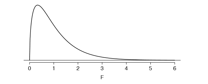
The larger the observed variability in the sample means (MSG) relative to the withingroup observations (MSE), the larger F will be and the stronger the evidence against the null hypothesis. Because larger values of F represent stronger evidence against the null hypothesis, we use the upper tail of the distribution to compute a p-value.
The F statistic and the F test
Analysis of variance (ANOVA) is used to test whether the mean outcome differs across 2 or more groups. ANOVA uses a test statistic F, which represents a standardized ratio of variability in the sample means relative to the variability within the groups. If H0 is true and the model assumptions are satisfied, the statistic F follows an F distribution with parameters \(df_1 = k -1 \) and \(df_2 = n - k\). The upper tail of the F distribution is used to represent the p-value.
Exercise \(\PageIndex{1}\)
The test statistic for the baseball example is F = 1.994. Shade the area corresponding to the p-value in Figure 5.29. 32
Example \(\PageIndex{1}\)
A common method for preparing oxygen is the decomposition
Example 5.42 The p-value corresponding to the shaded area in the solution of Exercise 5.41 is equal to about 0.115. Does this provide strong evidence against the null hypothesis?
The p-value is larger than 0.05, indicating the evidence is not strong enough to reject the null hypothesis at a signi cance level of 0.05. That is, the data do not provide strong evidence that the average on-base percentage varies by player's primary field position.
Reading an ANOVA table from software
The calculations required to perform an ANOVA by hand are tedious and prone to human error. For these reasons, it is common to use statistical software to calculate the F statistic and p-value.
An ANOVA can be summarized in a table very similar to that of a regression summary, which we will see in Chapters 7 and 8. Table 5.30 shows an ANOVA summary to test whether the mean of on-base percentage varies by player positions in the MLB. Many of these values should look familiar; in particular, the F test statistic and p-value can be retrieved from the last columns.
| DF | Sum Sq | Mean Sq | F value | Pr(> F) | |
|---|---|---|---|---|---|
|
position Residuals |
3 323 |
0.0076 0.4080 |
0.0025 0.0013 |
1.9943 |
0.1147 |
Graphical Diagnostics for an ANOVA Analysis
There are three conditions we must check for an ANOVA analysis: all observations must be independent, the data in each group must be nearly normal, and the variance within each group must be approximately equal.
- Independence. If the data are a simple random sample from less than 10% of the population, this condition is satisfied. For processes and experiments, carefully consider whether the data may be independent (e.g. no pairing). For example, in the MLB data, the data were not sampled. However, there are not obvious reasons why independence would not hold for most or all observations.
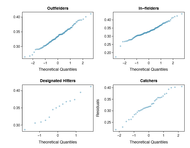
- Approximately normal. As with one- and two-sample testing for means, the normality assumption is especially important when the sample size is quite small. The normal probability plots for each group of the MLB data are shown in Figure 5.31; there is some deviation from normality for in elders, but this isn't a substantial concern since there are about 150 observations in that group and the outliers are not extreme. Sometimes in ANOVA there are so many groups or so few observations per group that checking normality for each group isn't reasonable. See the footnote33 for guidance on how to handle such instances.
- Constant variance. The last assumption is that the variance in the groups is about equal from one group to the next. This assumption can be checked by examining a sideby-side box plot of the outcomes across the groups, as in Figure 5.28 on page 239. In this case, the variability is similar in the four groups but not identical. We see in Table 5.27 on page 238 that the standard deviation varies a bit from one group to the next. Whether these differences are from natural variation is unclear, so we should report this uncertainty with the nal results.
33First calculate the residuals of the baseball data, which are calculated by taking the observed values and subtracting the corresponding group means. For example, an out elder with OBP of 0.435 would have a residual of \(0.405 - \bar {x}_{OF} = 0.071\). Then to check the normality condition, create a normal probability plot using all the residuals simultaneously.
Caution: Diagnostics for an ANOVA analysis
Independence is always important to an ANOVA analysis. The normality condition is very important when the sample sizes for each group are relatively small. The constant variance condition is especially important when the sample sizes differ between groups.
Multiple comparisons and controlling Type 1 Error rate
When we reject the null hypothesis in an ANOVA analysis, we might wonder, which of these groups have different means? To answer this question, we compare the means of each possible pair of groups. For instance, if there are three groups and there is strong evidence that there are some differences in the group means, there are three comparisons to make: group 1 to group 2, group 1 to group 3, and group 2 to group 3. These comparisons can be accomplished using a two-sample t test, but we use a modi ed signi cance level and a pooled estimate of the standard deviation across groups. Usually this pooled standard deviation can be found in the ANOVA table, e.g. along the bottom of Table 5.30.
| Class i | A | B | C |
|---|---|---|---|
|
\(n_i\) \(\bar {x}_i\) \(s_i\) |
58 75.1 13.9 |
55 72.0 13.8 |
51 78.9 13.1 |
Example \(\PageIndex{1}\)
A common method for preparing oxygen is the decomposition
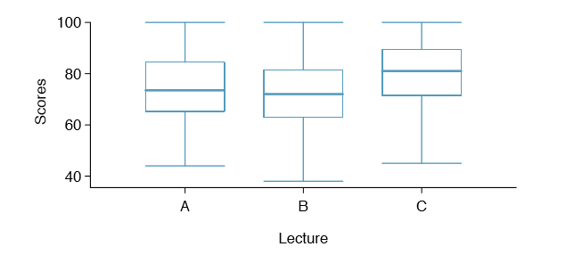
Example 5.43 Example 5.34 on page 236 discussed three statistics lectures, all taught during the same semester. Table 5.32 shows summary statistics for these three courses, and a side-by-side box plot of the data is shown in Figure 5.33. We would like to conduct an ANOVA for these data. Do you see any deviations from the three conditions for ANOVA?
In this case (like many others) it is difficult to check independence in a rigorous way. Instead, the best we can do is use common sense to consider reasons the assumption of independence may not hold. For instance, the independence assumption may not be reasonable if there is a star teaching assistant that only half of the students may access; such a scenario would divide a class into two subgroups. No such situations were evident for these particular data, and we believe that independence is acceptable.
The distributions in the side-by-side box plot appear to be roughly symmetric and show no noticeable outliers.
The box plots show approximately equal variability, which can be veri ed in Table 5.32, supporting the constant variance assumption.
Exercise \(\PageIndex{1}\)
A common method for preparing oxygen is the decompositio
Exercise 5.44 An ANOVA was conducted for the midterm data, and summary results are shown in Table 5.34. What should we conclude?34
34The p-value of the test is 0.0330, less than the default signi cance level of 0.05. Therefore, we reject the null hypothesis and conclude that the difference in the average midterm scores are not due to chance.
| Df | Sum Sq | Mean Sq | F value | Pr(>F) | |
|---|---|---|---|---|---|
|
lecture Residuals |
2 161 |
1290.11 29810.13 |
645.06 185.16 |
3.48 |
0.0330 |
There is strong evidence that the different means in each of the three classes is not simply due to chance. We might wonder, which of the classes are actually different? As discussed in earlier chapters, a two-sample t test could be used to test for differences in each possible pair of groups. However, one pitfall was discussed in Example 5.38 on page 238: when we run so many tests, the Type 1 Error rate increases. This issue is resolved by using a modi ed signi cance level.
Multiple comparisons and the Bonferroni correction for
The scenario of testing many pairs of groups is called multiple comparisons. The Bonferroni correction suggests that a more stringent signi cance level is more appropriate for these tests:
\[ \alpha ^* = \frac {\alpha}{K}\]
where K is the number of comparisons being considered (formally or informally). If there are k groups, then usually all possible pairs are compared and \(K = \frac {k(k - 1)}{2}\).
Example 5.45 In Exercise 5.44, you found strong evidence of differences in the average midterm grades between the three lectures. Complete the three possible pairwise comparisons using the Bonferroni correction and report any differences.
We use a modi ed signi cance level of \(\alpha ^* = \frac {0.05}{3} = 0.0167\). Additionally, we use the pooled estimate of the standard deviation: \(s_{pooled} = 13.61\) on df = 161, which is provided in the ANOVA summary table.
Lecture A versus Lecture B: The estimated difference and standard error are, respectively,
\[\bar {x}_A - \bar {x}_B = 75.1 - 72 = 3.1 SE = \sqrt {\frac {13.61^2}{58} +\frac {13.61^2}{55}} = 2.56\]
(See Section 5.4.4 on page 235 for additional details.) This results in a T score of 1.21 on df = 161 (we use the df associated with spooled). Statistical software was used to precisely identify the two-tailed p-value since the modi ed signi cance of 0.0167 is not found in the t table. The p-value (0.228) is larger than \(\alpha ^* = 0.0167\), so there is not strong evidence of a difference in the means of lectures A and B.
Lecture A versus Lecture C: The estimated difference and standard error are 3.8 and 2.61, respectively. This results in a T score of 1.46 on df = 161 and a two-tailed p-value of 0.1462. This p-value is larger than \(\alpha^*\), so there is not strong evidence of a difference in the means of lectures A and C.
Lecture B versus Lecture C: The estimated difference and standard error are 6.9 and 2.65, respectively. This results in a T score of 2.60 on df = 161 and a two-tailed p-value of 0.0102. This p-value is smaller than \(\alpha^*\). Here we nd strong evidence of a difference in the means of lectures B and C.
We might summarize the ndings of the analysis from Example 5.45 using the following notation:
\[\mu_A \overset {?} {=} \mu _B \mu _A \overset {?} {=} \mu _C \mu_B \ne \mu_C\]
The midterm mean in lecture A is not statistically distinguishable from those of lectures B or C. However, there is strong evidence that lectures B and C are different. In the first two pairwise comparisons, we did not have sufficient evidence to reject the null hypothesis. Recall that failing to reject H0 does not imply H0 is true.
Caution: Sometimes an ANOVA will reject the null but no groups will have statistically signi cant differences
It is possible to reject the null hypothesis using ANOVA and then to not subsequently identify differences in the pairwise comparisons. However, this does not invalidate the ANOVA conclusion. It only means we have not been able to successfully identify which groups differ in their means.
The ANOVA procedure examines the big picture: it considers all groups simultaneously to decipher whether there is evidence that some difference exists. Even if the test indicates that there is strong evidence of differences in group means, identifying with high con dence a specific difference as statistically signi cant is more difficult.
Consider the following analogy: we observe a Wall Street firm that makes large quantities of money based on predicting mergers. Mergers are generally difficult to predict, and if the prediction success rate is extremely high, that may be considered sufficiently strong evidence to warrant investigation by the Securities and Exchange Commission (SEC). While the SEC may be quite certain that there is insider trading taking place at the firm, the evidence against any single trader may not be very strong. It is only when the SEC considers all the data that they identify the pattern. This is effectively the strategy of ANOVA: stand back and consider all the groups simultaneously.