Regression diagnostics for one predictor

Last updated
Save as PDF

Page ID: 237

$ \newcommand{\vecs}[1]{\overset { \scriptstyle \rightharpoonup} {\mathbf{#1}} } $ $ \newcommand{\vecd}[1]{\overset{-\!-\!\rightharpoonup}{\vphantom{a}\smash {#1}}} $$\newcommand{\id}{\mathrm{id}}$ $ \newcommand{\Span}{\mathrm{span}}$ $ \newcommand{\kernel}{\mathrm{null}\,}$ $ \newcommand{\range}{\mathrm{range}\,}$ $ \newcommand{\RealPart}{\mathrm{Re}}$ $ \newcommand{\ImaginaryPart}{\mathrm{Im}}$ $ \newcommand{\Argument}{\mathrm{Arg}}$ $ \newcommand{\norm}[1]{\| #1 \|}$ $ \newcommand{\inner}[2]{\langle #1, #2 \rangle}$ $ \newcommand{\Span}{\mathrm{span}}$ $\newcommand{\id}{\mathrm{id}}$ $ \newcommand{\Span}{\mathrm{span}}$ $ \newcommand{\kernel}{\mathrm{null}\,}$ $ \newcommand{\range}{\mathrm{range}\,}$ $ \newcommand{\RealPart}{\mathrm{Re}}$ $ \newcommand{\ImaginaryPart}{\mathrm{Im}}$ $ \newcommand{\Argument}{\mathrm{Arg}}$ $ \newcommand{\norm}[1]{\| #1 \|}$ $ \newcommand{\inner}[2]{\langle #1, #2 \rangle}$ $ \newcommand{\Span}{\mathrm{span}}$$\newcommand{\AA}{\unicode[.8,0]{x212B}}$

Diagnostics for predictor
Diagnostics for residuals
1. Some important properties
2. Model departures that can be studied by residuals plots
Diagnostic plot
Contributors

Diagnostics for predictor

Diagnostic information about the predictor variable X, e.g. whether there are any outlying value, the range and concentration of X, are useful information that can provide clues to the appropriateness of the regression model assumptions.

For moderate-size data, we can use the stem-and leaf plot, or the dot plot to gather information about the range and concentration of the data, as well as the possible extreme values of X. Similar information can be extracted from a summary plot like the box plot.
If the data are observed over time, then both the predictor Y and the response X may show some pattern over time. A useful way of gathering this information is through the sequence plot (X values plotted against time).

To illustrate the effect of an extreme X value, consider the following example:

$$n = 16 , \sum_{i=1}^{n-1} X_i = 90, \sum_{i=1}^{n-1}Y_i = 330, \sum_{i=1}^{n-1}X_i^2 = 1000, \sum_{i=1}^{n-1}X_iY_i = 2400, X_n = 22, Y_n = 22.$$

Let $$\overline{X}_{n-1} = \sum_{i=1}^{n-1} X_i/(n-1) = 6, and \overline{Y}_{n-1} = \sum_{i=1}^{n-1} Y_i/(n-1) = 22.$$

Also,$$\sum_{i=1}^{n-1} (X_i - \overline{X}_{n-1})(Y_i - \overline{Y}_{n-1}) = \sum_{i=1}^{n-1} X_i Y_i - (n-1) \overline{X}_{n-1} \overline{Y}_{n-1} = 2400 - 15 \times 6\times 22= 420.$$
$$\sum_{i=1}^{n-1}(X_i - \overline{X}_{n-1})^2 = \sum_{i=1}^{n-1}X_i^2 - (n-1)(\overline{X})^2 = 1000 - 15 \times 6^2 = 460.$$

Hence, denoting by $b_1^{(n-1)}$ the least squares estimate of $\beta_1$ computed from the first n-1 observations, we have $$b_1^{(n-1)} = \frac{\sum_{i=1}^{n-1} (X_i - \overline{X}_{n-1})(Y_i - \overline{Y}_{n-1})}{\sum_{i=1}^{n-1}(X_i - \overline{X}_{n-1})^2} = \frac{420}{460} = 0.913.$$ For the whole data set, $$\overline{X} = (\sum_{i=1}^{n-1} X_i + X_n)/n = 7. \overline{Y} = (\sum_{i=1}^{n-1} Y_i + Y_n)/n = 22.$$

$$\sum_{i=1}^n (X_i - \overline{X})(Y_i - \overline{Y}) = \sum_{i=1}^n X_i Y_i - n \overline{X}\overline{Y} = (2400+22\times 22) - 16 \times 7 \times 22 = 420.$$
$$\sum_{i=1}^n (X_i - \overline{X})^2 = \sum_{i=1}^n X_i^2 - n(\overline{X})^2 = (1000+20^2) - 16 \times 7^2 = 616.$$

So, from the full data, estimate for $\beta_1$ is $b_1 =\frac{\sum_{i=1}^n (X_i - \overline{X})(Y_i - \overline{Y})}{
\sum_{i=1}^n (X_i - \overline{X})^2} = \frac{420}{616} = 0.6818.$ Note that, in this example, standard deviation of X estimated from
the first n-1 observations is $s_X^{(n-1)} = \sqrt{\frac{1}{n-2}\sum_{i=1}^{n-1}(X_i - \overline{X}_{n-1})^2} = 5.73$. And observe that $X_n > \overline{X}_{n-1} + 2 s_X^{(n-1)}.$
It can be shown that if we use $b_0^{(n-1)}$ to denote the least squares estimate of $\beta_0$, from the first n-1 observations,
and $e_n^{(n-1)} = Y_n - b_0^{(n-1)} - b_1^{(n-1)} X_n$, then $b_1 = b_1^{(n-1)} + \frac{(1-\frac{1}{n})(X_n - \overline{X}_{n-1})e_n^{(n-1)}}{\sum_{i=1}^n (X_i - \overline{X})^2} = b_1^{(n-1)} + \frac{(X_n - \overline{X})}{\sum_{i=1}^n (X_i - \overline{X})^2}e_n^{(n-1)}.$

Diagnostics for residuals

Residuals $e_i = Y_i - \widehat Y_i$ convey information about the appropriateness of the model. In particular, possible departures from model assumptions are often reflected in the plot of residuals against either predictor(s) or fitted values, or in the distribution of the residuals.

Some important properties

Mean : We have seen that $\sum_i e_i =0$ and hence = $\overline{e} =\frac{1}{n}\sum_i e_i = 0.$

Variance : Var $(e) = s^2 = \frac{1}{n-2}\sum_i(e_i - \overline{e})^2 = \frac{1}{n-2}\sum_i e_i^2 = MSE.$

Correlations : $\sum_i X_i e_i = 0, \sum_i \widehat Y_i e_i =0$ and $\overline{e} =0$ imply that Corr$(X,e) =0$ and Corr$(\widehat Y,e) = 0.$

Nonindependence : The residuals $e_i$ are not independent even if the model errors $\varepsilon_i$ are. This is because the $e_i$'s satisfy two constraints: $\sum_i e_i =0$ and $\sum_i X_i e_i =0.$ However, when n is large, the residuals are almost independent if the model assumptions hold.

Semi-studentized residuals : Standardize the residuals by dividing through by $\sqrt{MSE}$ to get the semi-studentized

residuals:
$$e_i^* = \frac{e_i - \overline{e}}{\sqrt{MSE}} = \frac{e_i}{\sqrt{MSE}}.$$

Model departures that can be studied by residuals plots

The regression function is not linear.
The error terms do not have a constant variance.
The error terms are not independent.
The model fits all but one or a few outliers.
The error terms are not normally distributed.
One or several predictor variables have been omitted from the model.

Diagnostic plot

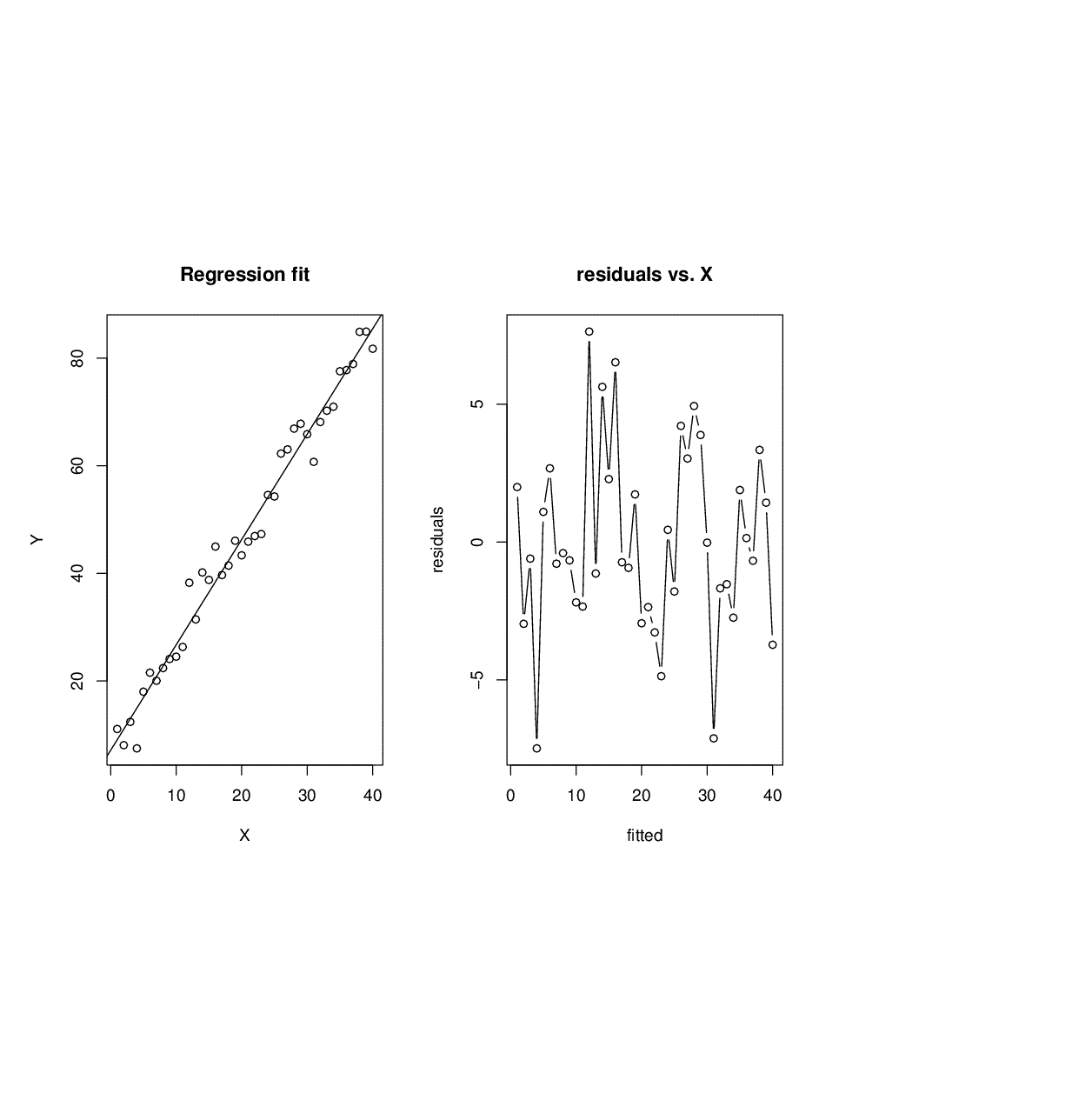
Plot of residuals versus time: When the observations involve a time component, the sequence plot, i.e. plot of residuals versus time are helpful in detecting possible pressence of runs or cycles. Runs may indicate that the errors are correlated in time. Systematic patterns like cycles may indicate presence of seasonality in the data.

Example: True model : Y = 5 + 2X + sin(X/10) + $\varepsilon$, where X is the time, and $\varepsilon$ ~ N(0,9). $X_i$ = i for i = 1,2,...,40. Fitted linear regression model for simulated data:

Coefficients	Estimate	Std. Error	t-statistic	P-value
Intercept	7.0878	1.1035	6.423	1.5 x 10^-7
Slope	1.9598	0.0469	41.783	< 2 x 10^-16

$\sqrt{MSE}$ = 3.424. R² = 0.9787, $R_{ad}^2$ = 0.9781.

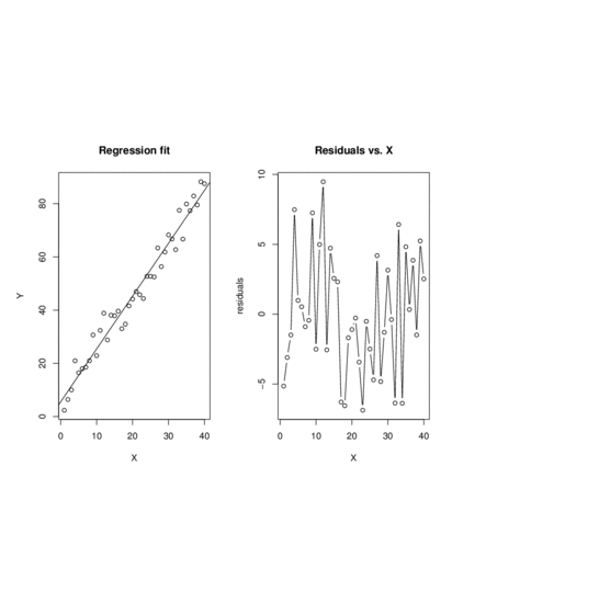
Another example of time course data

True model : Y = 5 + 3X + 3sin(X/5) + $\varepsilon$. 40 observations at $X_i$ = i, i = 1,...,40. $\varepsilon$ sin N(0,9). The linear model fit is given below.

Coefficients	Estimate	Std. Error	t-statistic	P-value
Intercept	5.5481	1.14164	3.917	0.000361
Slope	1.9862	0.0602	32.991	< 2 x 10^-16

$\sqrt{MSE}$ = 4.395. R² = 0.9663, $R_{ad}^2$ = 0.9654.

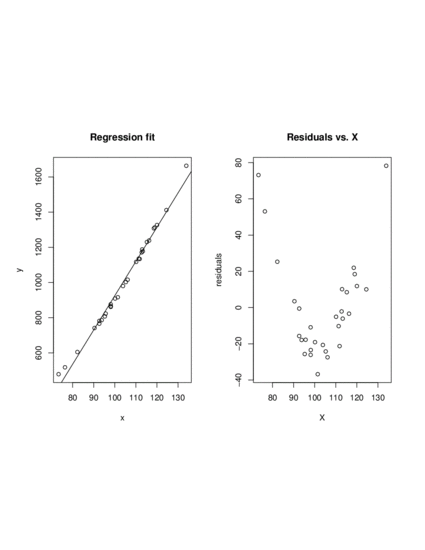
Nonlinearity of the regression function : If the plot of the residuals versus predictors show discernible, nonlinear pattern, that is an indication of possible nonlinearity if the regression function.

Example :True model : Y = 5 - X + 0.1 * X² + $\varepsilon$ with $\varepsilon$ ~ N(0, (10)²). We simulate 30 observations with X following a N(100, (16)²) distribution. The data summary is given below.

$\overline{X} = 104.13, \overline{Y} = 1004.79, \sum_i X_i^2 = 330962.9, \sum_i Y_i^2 = 32466188, \sum_i X_iY_i = 3249512.$

The linear model : Y = $\beta_0 + \beta_1 X + \epsilon$ was fitted to this data. The following table gives the summary.

Coefficients	Estimate	Std. Error	t-statistic	P-value
Intercept	-1021.3803	40.0648	-25.49	< 2 x 10^-16
Slope	19.4587	0.3814	51.01	< 2 x 10^-16

$\sqrt{MSE}$ = 28.78. R² = 0.9894, $R_{ad}^2$ = 0.989.

Presence of outliers : If some of the semi-studentized residuals have "too large" absolute values (say $|e_i^*|$ > 3 for some i) then the corresponding observation can be taken to be an outlier (in Y).

Contributors

Yingwen Li
Debashis Paul