Two Factor ANOVA Under Balanced Designs
- Page ID
- 210

The dependence of a response variable on two factors, A and B, say, is of interest.
- Factor A has a levels and Factor B has b levels.
- In total there are a x b treatments.
- Sample sizes for all treatment groups are equal (balanced design).
-
Goal: to study the simultaneous effects of the two factors on the response variable, including their respective main effects and their interaction effects.
1.1 Example: drugs for hypertension
A medical investigator studied the relationship between the response to three blood pressure lowering drugs for hypertensive males and females. The investigator selected 30 males and 30 females and randomly assigned 10 males and 10 females to each of the three drugs.
- This is a balanced randomized complete block design (RCBD)
- Two factors:
- A - gender (observational factor)
- B - drug (experimental factor)
- Factor A has a = 2 levels: male vs. female
- Factor B has b = 3 levels: drug 1, drug 2, and drug 3
- In total there are a x b = 2 x 3 = 6 treatments
- For each treatment, the sample size is n = 10
| Treatment | Description | Sample Size |
| 1 | drug 1, male | 10 |
| 2 | drug 1, female | 10 |
| 3 | drug 2, male | 10 |
| 4 | drug 2, female | 10 |
| 5 | drug 3, male | 10 |
| 6 | drug 3, female | 10 |
1.2 Population means
- Treatment means: \(\mu_{ij}\) = population mean response of the treatment with factor A at level i and factor B at level j
- Factor level means: \(\mu_{i\cdot}\) = population mean response when the i-th level of factor A is applied; \(\mu_{\cdot j}\) = population mean response when the j-th level of factor B is applied:
- Overall mean (the basic line quantity in comparisons of factor effects):
| FACTOR B | ||||||
| j = 1 | j = 2 | . . . . . | j = b | Row Avg | ||
| i = 1 | \(\mu_{11}\) | \(\mu_{12}\) | . . . . . | \(\mu_{1b}\) | \(\mu_{1\cdot}\) | |
| i = 2 | \(\mu_{21}\) | \(\mu_{22}\) | . . . . . | \(\mu_{2b}\) | \(\mu_{2\cdot}\) | |
| FACTOR A | . | . . . | . . . | . . . . . | . . . | . . . |
| i = a | \(\mu_{a1}\) | \(\mu_{a2}\) | . . . . . | \(\mu_{ab}\) | \(\mu_{a\cdot}\) | |
| Column Avg | \(\mu_{\cdot 1}\) | \(\mu_{\cdot 2}\) | . . . . . | \(\mu_{\cdot b}\) | \(\mu_{\cdot \cdot}\) |
1.3 Main effects
- Main effects are defined as the differences between factor level means and the overall mean
- Factor A main effects: \(\alpha_{i}\) = main effect of factor A at the i-th factor level

- Factor B main effects: \(\beta_{j}\) = main effect of factor B at the j-th factor level
.gif?revision=1)
- For both factor A and factor B, the sum of main effects is zero
1.4 Interaction effects
- Interaction effects describe how the effects of one factor depend on the levels of the other factor
- \((\alpha\beta)_{ij}\) = interaction effect of the i-th level of factor A and j-th level of factor B
.gif?revision=1)
- Note: for \(1 \leq i \leq a, 1\leq j \leq b\)
- If all \((\alpha\beta)_{ij} = 0, i = 1, ..., a, j = 1, ..., b\), then the factor effects are additive
- This is equivalent to
- If at least one of the \((\alpha\beta)_{ij}\)'s is nonzero, then the factor effects are interacting
- This means that the effects of one factor are different for differing levels of the other factor.
1.5 Additive factor effects
- If the two are additive (i.e. no interaction)
- Each factor can be studied separately, based on their factor level means \(\{\mu_{i\cdot}\}\) and \(\{\mu_{\cdot j}\}\), respectively
- This is much simpler than the joint analysis based on the treatment means \(\{\mu_{ij}\}\)
Example 1
Factor A has a = 2 levels, Factor B has b = 3
- Check additivity for all pairs of (i,j)
\[\alpha_{1} = \mu_{1\cdot} - \mu_{\cdot \cdot} = 12 - 12 = 0\]
\[\beta_{1} = \mu_{\cdot 1} - \mu_{\cdot \cdot} = 9 - 12 = -3\]
\[\mu_{11} = 9\]
\[\mu_{\cdot \cdot} + (\alpha_{1} + \beta_{1}) = 12 + (0 - 3) = 9 = \mu_{11}\]
- Exercise: Complete the check for additivity
| FACTOR B | |||||
| j = 1 | j = 2 | j = 3 | \(\mu_{i\cdot}\) | ||
| FACTOR A | i = 1 | 9 | 11 | 16 | 12 |
| i = 2 | 9 | 11 | 16 | 12 | |
| \(\mu_{\cdot j}\) | 9 | 11 | 16 | 12 (= \(\mu_{\cdot \cdot}\)) |
1.6 Graphical method: interaction plots
Interaction plots constitute a graphical tool to check additivity.- X-axis is for the factor A (or B) levels, and Y-axis is for the treatment means \(\mu_{ij}\)'s
- seperate curves are drawn for each of the factor B (or A) levels

- If the curves are all horizontal, then the factor on the X-axis has no effect at all, i.e. the treatment means do not depend on the level of that factor
- If the curves are overlapping, then the other factor (the one not on the X-axis) has no effect
- If the curves are parallel, then the two factors are additive, i.e. the effects of factor A do not depend on (or interact with) the level of factor B, and vice versa
- Note: "horizontal" and "overlapping" are special cases of "parallel"
For Example 1:
- The two factors are additive
- Moreover, factor A does not have any effect at all (main effects of factor A are all zero)
- Factor B does have some effects (not all main effects of factor B are zero)
| Factor B | |||||
| j = 1 | j = 2 | j = 3 | \(\mu_{i\cdot}\) | ||
| Factor A | i = 1 | 11 | 13 | 18 | 14 |
| i = 2 | 7 | 9 | 14 | 10 | |
| \(\mu_{\cdot j}\) | 9 | 11 | 16 | 12 (=\(\mu_{\cdot \cdot}\)) |

- The two factors are additive, since the curves are parallel
- Both factors have some effects (main effects of both factors are not all zero), since the curves are neither horizontal to the X-axis nor overlapping in any of the plots
- Note: Indeed, you only need to examine one of the two plots. If the curves in one plot are parallel, the curves in the other plot must also be parallel
Summary: Additive Model
- For all pairs of (i, j): \(\mu_{ij} = \mu_{\cdot \cdot} + \alpha_{i} + \beta_{j}\)
- The curves in an interaction plot are parallel
- The difference between treatments means for any two levels of factor B (respectively, A) is the same for all level of factor A (respectively, B):
\[\mu_{1j} - \mu_{1j'} = ... = \mu_{aj} - \mu_{aj'}, 1 \leq j, j' \leq b\]
1.7 Interacting factor effects
- Interpretation of \((\alpha\beta)_{ij}\): the difference between the treatment mean \(\mu_{ij}\) and the value that would be expected if the two factors were additive
- Factor A and factor B are interacting: if some \((\alpha\beta)_{ij} \neq 0\), i.e. \(\mu_{ij} \neq \mu_{\cdot \cdot} + \alpha_{i} + \beta_{j}\) for some (i, j)
- Equivalently, the curves are not parallel in an interaction plot
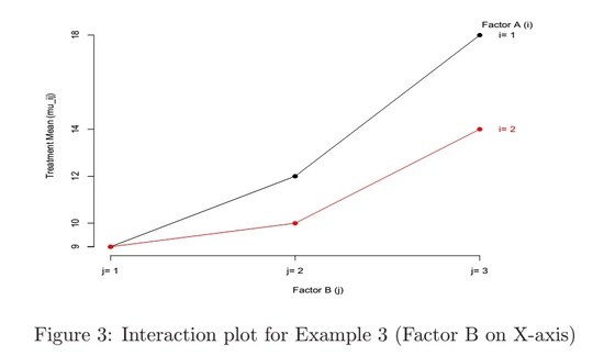
Example 3
Factor A: a = 2 levels; Factor B: b = 3 levels
| Factor B | |||||
| j = 1 | j = 2 | j = 3 | \(\mu_{i\cdot}\) | ||
| Factor A | i = 1 | 9 | 12 | 18 | 13 |
| i = 2 | 9 | 10 | 14 | 11 | |
| \(\mu_{\cdot j\) | 9 | 11 | 16 | 12 (=\(\mu_{\cdot \cdot}\)) |
- The two curves in the interaction plot are not parallel, which means the two factors are interacting
- For example:
\[\alpha_{1} = \mu_{1\cdot} - \mu_{\cdot \cdot} = 13 - 12 = 1 and \beta_{1} = \mu_{\cdot 1} - \mu_{\cdot \cdot} = 9 - 12 = -3\]
\[Thus 9 = \mu_{11} \neq \mu_{\cdot \cdot} + \alpha_{1} + \beta_{1} = 12 + 1 - 3 = 10\]
\[Or (\alpha\beta)_{11} = 9 - 10 = -1 \neq 0\]
\[\mu_{11} - \mu_{12} = 9 - 12 = -3 \neq \mu_{21} - \mu_{22} = 9 - 10 = -1\]
- There is a larger difference among treatment means between the two levels of factor A when factor B is at the 3rd level (j = 3) than when B is at the first two levels (j = 1, 2)
 Summary: Interactions
 Suppose we put Factor B on the X-axis of the interaction plot
- The differences in heights of the curves reflect Factor A effects. On the other hand, if all curves are overlapping, then Factor A has no effect.
- The departure from horizontal by the curves reflects Factor B effects. On the other hand, if all curves are horizontal, then Factor B has no effect.
- The lack of parallelism among the curves reflects interaction effects.
- Any one factor with no effect means additivity
- Important: no main effects does not necessarily mean no effects or no interaction effects.
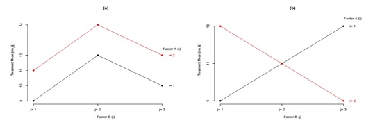
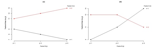
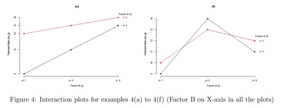
Example 4 (refer to figure 4)
- Figure (a): additive
- Figure (b) and (c): Factor B has no main effects, but Factor A and Factor B are interacting
- Figure (d): when Factor A is at level 1, treatment means increase with Factor B levels; when Factor A is at level 2, the trend becomes decreasing
- Figure (e): larger difference among treatment means between the two levels of Factor A when Factor B is at a smaller indexed level
- Figure (f): more dramatic change of treatment means among Factor B levels when Factor A is at level 1