15.4: Practice Regression of Health and Happiness

Our first practice will include the whole process to calculate all of the equations and the ANOVA Summary Table.

Scenario

In this scenario, researchers are interested in explaining differences in how happy people are based on how healthy people are. They gather quantitative data on each of these variables from 18 people and fit a linear regression model (another way to say that they constructed a regression line equation) to explain the variability of one variable (say, happiness) based on the variability of the other variable (health). We will follow the four-step hypothesis testing procedure to see if there is a relation between these variables that is statistically significant.

Step 1: State the Hypotheses

What do you think?  Do you think that happiness and health vary in the same direction, in opposite directions, or do not vary together?  This sounds like the set up for a research hypothesis for a correlation, and it is!  The small change here is that we're focusing on the slope (\(b\) or beta) of the line, rather merely testing if there is a linear relationship.

Example \(\PageIndex{1}\)

What could be a research hypothesis for this scenario?  State the research hypothesis in words and symbols.

Solution

The research hypothesis should probably be something like, "There will be a positive slope in the regression line for happiness and health."  

Symbols:  \( \beta > 0 \)

For right now, we haven't made it clear which might be our predictor variable and which might be our criterion variable, the outcome. If we decide that health is the predictor and happiness is the outcome, we could add that we think that changes in health predict changes in happiness.  It seems reasonable in this situation to reverse the IV and DV here, and say that change in happiness could also predict changes in health.  There's data to support both of these ideas!

The null hypothesis in regression states that there is no relation between our variables so you can't use one variable to predict or explain the other variable. 

Example \(\PageIndex{2}\)

What is the null hypothesis for this scenario?  State the null hypothesis in words and symbols.  

Solution

The null hypothesis is that there is no relationship between health and happiness, so "The slope in the regression line for happiness and health will be zero." Neither variable can predict or explain the other variable.

Symbols: \( \beta = 0 \)

These hypothesis are not as clear-cut as we've previously had because regression analyses can show a lot.  If it's easier, you can fall back on the general hypothesis for correlations rather than focus on slopes.  However, that misses the addition information that regressions also show:  How much variability in one variable is due to the other variable.

Step 2: Find the Critical Value

Because regression and ANOVA are the same analysis, our critical value for regression will come from the same place: the Table of Critical Values of F (found in the first chapter discussing ANOVAs, or found through the Common Critical Values page at the end of the book). 

The ANOVA Summary Table used for regression uses two types of degrees of freedom. We previously saw that the Degrees of Freedom for our numerator, the Model line, is always 1 in a linear regression, and that the denominator degrees of freedom, from the Error line, is \(N – 2\).

In this instance, we have 18 people so our degrees of freedom for the denominator is 16. Going to our \(F\) table, we find that the appropriate critical value for 1 and 16 degrees of freedom is F_Critical = 4.49.  Isn't it nice to do the simple things that we learned about seemingly eons ago?

Step 3: Calculate the Test Statistic

The process of calculating the test statistic for regression first involves computing the parameter estimates for the line of best fit. To do this, we first calculate the means, standard deviations, and sum of products for our variables, as shown in Table \(\PageIndex{1}\).  

Table \(\PageIndex{1}\): Raw Scores in Empty Sum of Products Table

Health	Difference: Health - Mean	Health Difference Squared	Happiness	Difference: Happiness - Mean	Happiness Difference Squared	Health Diff * Happy Diff
16.99			16.38
17.42			16.89
17.65			10.36
18.21			18.49
18.28			14.26
18.30			15.23
18.39			12.08
18.63			17.57
18.89			21.96
19.45			21.17
19.67			18.12
19.91			17.86
20.35			18.74
21.89			17.71
22.48			17.11
22.61			16.47
23.25			21.66
23.65			22.13
\(\sum = 356.02 \)	\(\sum = ? \)	\(\sum = ? \)	\(\sum = 314.18 \)	\(\sum = ? \)	\(\sum = ? \)	\(\sum = ? \)

This table should look pretty familiar, as it's the same as the one we used to calculate a correlation when we didn't have have the standard deviation provided.  

First things first, let's find the means so that we can start filling in this table.

Exercise \(\PageIndex{1}\)

What is the average score for the Health variable?  What is the average score for the Happiness variable?

Answer

\[ \bar{X}_{Hth} = \dfrac{\sum X}{N} = \dfrac{356.02}{18} = 19.78 \nonumber \]

\[ \bar{X}_{Hpp} = \dfrac{\sum X}{N} = \dfrac{314.19}{18} = 17.46  \nonumber \]

Now that we have the means, we can fill in the complete Sum of Products table.

Exercise \(\PageIndex{2}\)

Fill in Table \(\PageIndex{1}\) by finding the differences of each score from that variable's mean, squaring the differences, multiplying them, then finding the sums of each of these.

Answer

Table \(\PageIndex{2}\)- Completed Sum of Products Table

Health	Difference: Health - Mean	Health Difference Squared	Happiness	Difference: Happiness - Mean	Happiness Difference Squared	Health Diff * Happy Diff
16.99	-2.79	7.78	16.38	-1.08	1.17	3.01
17.42	-2.36	5.57	16.89	-0.57	0.32	1.35
17.65	-2.13	4.54	10.36	-7.10	50.41	15.12
18.21	-1.57	2.46	18.49	1.03	1.06	-1.62
18.28	-1.50	2.25	14.26	-3.20	10.24	4.80
18.30	-1.48	2.19	15.23	-2.23	4.97	3.30
18.39	-1.39	1.93	12.08	-5.38	28.94	7.48
18.63	-1.15	1.32	17.57	0.11	0.01	-0.13
18.89	-0.89	0.79	21.96	4.50	20.25	-4.01
19.45	-0.33	0.11	21.17	3.71	13.76	-1.22
19.67	-0.11	0.01	18.12	0.66	0.44	-0.07
19.91	0.13	0.02	17.86	0.40	0.16	0.05
20.35	0.57	0.32	18.74	1.28	1.64	0.73
21.89	2.11	4.45	17.71	0.25	0.06	0.53
22.48	2.70	7.29	17.11	-0.35	0.12	-0.95
22.61	2.83	8.01	16.47	-0.99	0.98	-2.80
23.25	3.47	12.04	21.66	4.20	17.64	14.57
23.65	3.87	14.98	22.13	4.67	21.81	18.07
\(\sum = 356.02 \)	\(\sum = -0.02 \)	\(\sum = 76.07 \)	\(\sum = 314.18 \)	\(\sum = -0.09 \)	\(\sum = 173.99 \)	\(\sum = 58.22 \)

 

In Table \(\PageIndex{2}\), the difference scores for each variable (each score minus the mean for that variable) sum to nearly zero, so all is well there.  Let's use the sum of those squares to calculate the standard deviation for each variable.  

Example \(\PageIndex{3}\)

Calculate the standard deviation of the Health variable.

Solution

Using the standard deviation formula:
\[s=\sqrt{\dfrac{\sum(X-\overline {X})^{2}}{N-1}} \nonumber \]
We can fill in the numbers from the table and N to get:
\[s_{Hth}=\sqrt{\dfrac{76.07}{18-1}} = \sqrt{\dfrac{76.07}{17 }}\nonumber \]
Some division, then square rooting to get:
\[s_{Hth}= \sqrt{4.47 }\nonumber \]
\[s_{Hth}= 2.11 \nonumber \]

If you used spreadsheet, you might get 2.12.  That's fine, but we'll use 2.11 for future calculations.  

Your turn!

Exercise \(\PageIndex{3}\)

Calculate the standard deviation of the Happiness variable.

Answer

\[s=\sqrt{\dfrac{\sum(X-\overline {X})^{2}}{N-1}} \nonumber \]
\[s_{Hpp}=\sqrt{\dfrac{173.99}{18-1}} = \sqrt{\dfrac{173.99}{17 }}\nonumber \]
\[s_{Hpp}= \sqrt{10.23 }\nonumber \]
\[s_{Hpp}= 3.20 \nonumber \]

Next up, we must calculate the slope of the line.  There are easier ways to show this if we start substituting names for symbols, but let's stick with the names of our variables in this formula:

\[\mathrm{b}=\dfrac{(Diff_{Hth} * Diff_{Hpp})}{Diff_{Hth}^2} =\dfrac{58.22}{76.07 }=0.77 \nonumber \]

What this equation is telling us to do is pretty simple once we have the Sum of Products table filled out.  We just take the sum of the multiplication of each of the differences (that's the most bottom most right cell in the table), and divide that by the sum of the difference scores squared for the Health variable.  The result means that as Health (\(X\)) changes by 1 unit, Happiness (\(Y\)) will change by 0.77. This is a positive relation.

Next, we use the slope, along with the means of each variable, to compute the intercept:  \(a =\overline{X_y}-b\overline{X_x} \)

Example \(\PageIndex{4}\)

Using the means and the slope (b) that we just calculated, calculate the intercept (a).

Solution

\[a =\overline{X_y}-b\overline{X_x} \nonumber \]
\[a =\overline{X}_{Hpp}-(b * \overline{X}_{Hth}) \nonumber \]
\[a =17.46-(0.77 * 19.78) \nonumber \]
\[a =17.46-(15.23 ) \nonumber \]
\[a =2.23 \nonumber \]

This number varies widely based on how many decimal points you save while calculating.  The numbers shown are when only two decimal points are used, which is the minimum that you should be writing down and saving.  

For this particular problem (and most regressions), the intercept is not an important or interpretable value, so we will not read into it further.

Now that we have all of our parameters estimated, we can give the full equation for our line of best fit:  \(\widehat{y} =\mathrm{a}+(\mathrm{b}*{X}) \)

Example \(\PageIndex{5}\)

Construct the regression line equation for the predicted Happiness score (\(\widehat{y}).

Solution

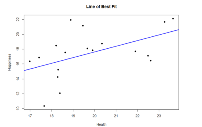
\[\widehat{y} = 2.23 + 0.77\text{x} \nonumber \]

It doesn't quite make sense yet, but you actually just answered many potential research questions!  We can also plot this relation in a scatterplot and overlay our line onto it, as shown in Figure \(\PageIndex{1}\).

Figure \(\PageIndex{1}\): Health and Happiness Data and Regression Line.  (CC-BY-NC-SA Foster et al. from An Introduction to Psychological Statistics)

We can use the regression line equation to find predicted values for each observation and use them to calculate our sums of squares for the Model and the Error, but this is tedious to do by hand, so we will let the computer software do the heavy lifting in that column of our ANOVA Summary Table in Table \(\PageIndex{3}\).

Table \(\PageIndex{3}\): ANOVA Summary Table with SS

Source	\(SS\)	\(df\)	\(MS\)	\(F\)
Model	44.62
Error	129.37			N/A
Total	173.99		N/A	N/A

Happily, the Total row is still the sum of the other two rows, so that was added, too.  Now that we have these, we can fill in the rest of the ANOVA table.

Example \(\PageIndex{6}\)

Fill in the rest of the ANOVA Summary Table from Table \(\PageIndex{3}\).

Solution

Table \(\PageIndex{4}\): ANOVA Summary Table with SS

Source	\(SS\)	\(df\)	\(MS\)	\(F\)
Model	44.62	1	\(MS_M = \dfrac{SS_M}{df_M} = \dfrac{44.62}{1} = 44.62 \)	\(F = \dfrac{MS_M}{MS_E} = \dfrac{44.62}{8.09} = 5.52\)
Error	129.37	\(N - 2 = 18 - 2 = 16\)	\(MS_E = \dfrac{SS_E}{df_E} = \dfrac{129.37}{16} = 8.09 \)	leave blank
Total	173.99	\(N - 1 = 18 - 1 = 17\)	leave blank	leave blank

Happily again, we can do a computation check to make sure that our Degrees of Freedom are correct since the sum of the Model's df and the Error's df should equal the Total df.  And since \(1 + 16 = 17\), we're doing well!

This gives us an obtained \(F\) statistic of 5.52, which we will now use to test our hypothesis.

Step 4: Make the Decision

We now have everything we need to make our final decision. Our calculated test statistic was \(F_{Calc} = 5.52\) and our critical value was \(F_{Crit} = 4.49\). Since our calculated test statistic is greater than our critical value, we can reject the null hypothesis because this is still true:

Note

Critical \(<\) Calculated \(=\) Reject null \(=\) There is a linear relationship. \(= p<.05 \)

Critical \(>\) Calculated \(=\) Retain null \(=\)  There is not a linear relationship. \(= p>.05\)

 

Write-Up:  Reporting the Results

We got here a sorta roundabout way, so it's hard to figure out what our conclusion should look like.  Let's start by including the four components needed for reporting results.  

Example \(\PageIndex{7}\)

Use the four components for reporting results to start your concluding paragraph:

1. The statistical test is preceded by the descriptive statistics (means). 
2. The description tells you what the research hypothesis being tested is. 
3. A "statistical sentence" showing the results is included. 
4. The results are interpreted in relation to the research hypothesis.

Solution

1. The average health score was 19.78.  The average happiness score was 17.46.
2. The research hypothesis was that here will be a positive slope in the regression line for happiness and health.
3. The ANOVA results were F(1,16)=5.52, p< .05.
4. The results are statistically significant, and the positive Sum or Products shows a positive slope so the research hypothesis is supported.

Let's add one more sentence for a nice little conclusion to our regression analysis:  We can predict levels of happiness based on how healthy someone is.  So, our final write-up could be something like:

We can predict levels of happiness (M=17.46) based on how healthy someone is (M=19.78) (F(1,16)=5.52, p< .05).  The average health score was 19.78.  The average happiness score was 17.46.  The research hypothesis was supported; there is a positive slope in the regression line for happiness and health.

Yep, that's pretty clunky.  As you learn more about regression (in future classes), the research hypotheses will make more sense.  

Accuracy in Prediction

We found a large, statistically significant relation between our variables, which is what we hoped for. However, if we want to use our estimated line of best fit for future prediction, we will also want to know how precise or accurate our predicted values are. What we want to know is the average distance from our predictions to our actual observed values, or the average size of the residual (\(Y − \widehat {Y}\)). The average size of the residual is known by a specific name: the standard error of the estimate (\(S_{(Y-\widehat{Y})}\)), which is given by the formula

\[S_{(Y-\widehat{Y})}=\sqrt{\dfrac{\sum(Y-\widehat{Y})^{2}}{N-2}} \nonumber \]

This formula is almost identical to our standard deviation formula, and it follows the same logic. We square our residuals, add them up, then divide by the degrees of freedom. Although this sounds like a long process, we already have the sum of the squared residuals in our ANOVA table! In fact, the value under the square root sign is just the \(SS_E\) divided by the \(df_E\), which we know is called the mean squared error, or \(MS_E\):

\[s_{(Y-\widehat{Y})}=\sqrt{\dfrac{\sum(Y-\widehat{Y})^{2}}{N-2}}=\sqrt{MS_E} \nonumber \]

For our example:

\[s_{(Y-\widehat{Y})}=\sqrt{\dfrac{129.37}{16}}=\sqrt{8.09}=2.84 \nonumber \nonumber \]

So on average, our predictions are just under 3 points away from our actual values.

There are no specific cutoffs or guidelines for how big our standard error of the estimate can or should be; it is highly dependent on both our sample size and the scale of our original \(Y\) variable, so expert judgment should be used. In this case, the estimate is not that far off and can be considered reasonably precise.

Clear as mud?  Let's try another practice problem!

Contributors and Attributions

• Foster et al. (University of Missouri-St. Louis, Rice University, & University of Houston, Downtown Campus)

• Dr. MO (Taft College)