14.7.2: Practice on Nutrition

This second example will use the same formula, more or less.  Instead of providing the standard deviations, you will need to calculate them.  This example uses nutrition data from fast food restaurants from www.OpenIntro.org. You should probably try the previous practice problem because it gives more hints than this one will. 

Scenario

When Dr. MO was on a low-carb diet, she noticed that things that were low in carbohydrates tended to be high in fat, and vice versa.  Now that she has the skills and the data set, we can test to see if there is a statistical relationship!  Our analysis will look at the chicken dishes from one fast food restaurant using the nutritional data from OpenIntro.org. 

Step 1: State the Hypotheses

What kind of linear relationship is it if it looks like as fat goes up, carbs go down? 

Exercise \(\PageIndex{1}\)

What is a research hypothesis for this scenario?

Answer

The research hypothesis should be:  There is negative linear relationship between fat and carbohydrates in the sample of chicken dishes from one fast food restaurant.

Sometimes, people will add a description of what the negative linear relationship would look like to their research hypothesis:        There is negative linear relationship between fat and carbohydrates in the sample of chicken dishes from one fast food restaurant such that foods with more fat tend to have fewer carbohydrates.

Let’s look at the scatterplot to see if it looks like a negative linear relationships (as one goes up, the other goes down), which should have a general linear trend from the top left to the bottom right.

Figure \(\PageIndex{1}\): Scatterplot of Carbohydrates by Fat for 13 Chicken Meals. (CC-BY; Michelle Oja via OpenIntro.org)

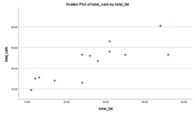
Uh-oh, already it looks like Dr. MO’s research hypothesis is not working out.  There does seem to be a general linear trend, but it does not look like a negative correlation; it actually looks like a positive correlation! 

Let’s state our null hypothesis so that we can get to the analysis to see what’s going on statistically. 

Exercise \(\PageIndex{2}\)

What is a null hypothesis for this scenario?

Answer

The null hypothesis should be:  There is no linear relationship between fat and carbohydrates in the sample of chicken dishes from one fast food restaurant.

Before we get too far into the weeds, let’s consider why a correlational analysis is the appropriate analysis.  Your first clue is the research hypothesis.  We are not comparing whether the average fat content is higher than the average carbohydrate content; in other words, we aren’t looking at mean differences.  Another clue is that we have means of two different variables, not means of two different groups.  So that leads to recognizing that we have two quantitative variables, not a quantitative variable that we measured for two or more groups (qualitative variables).  Whenever you’re not sure, check out the Decision Tree handout!

Step 2: Find the Critical Values

The critical values for correlations come from the Table of Critical Values of r again.  We were not given any information about the level of significance at which we should test our hypothesis, so we will assume \(α = 0.05\) as always. From the table, we can see that we need the Degrees of Freedom, which is N–2.  The data is provided below, (Table \(\PageIndex{1}\)) and shows that we have 13 chicken dishes that we are looking at.  With p=.05 level, the critical value for N –2  (13–2=11) is critical r-value is 0. 0.553.

Step 3: Calculate the Test Statistic

It’s easiest to calculate the standard deviation and Pearson’s r by using a table to do most of the calculations.  If we sum each column in the table, we also can easily find the mean. 

Table \(\PageIndex{1}\)- Raw Data for Sum of Products Table for Fat and Carbs

Item	Total Fat	Fat Difference:  Fat Minus Mean	Squared	Total Carbs	Carb Differences:  Carb Minus Mean	Squared	Fat Diff * Carb Diff
2 piece Prime-Cut Chicken Tenders	11			19
Chicken Tender 'n Cheese Slider	12			30
Buffalo Chicken Slider	13			31
3 piece Prime-Cut Chicken Tenders	17			28
Buttermilk Buffalo Chicken Sandwich	24			53
Crispy Chicken Farmhouse Salad	24			26
Buttermilk Crispy Chicken Sandwich	26			52
5 piece Prime-Cut Chicken Tenders	28			47
Bourbon BBQ Chicken Sandwich	31			66
Buttermilk Chicken Bacon & Swiss	31			56
Buttermilk Chicken Cordon Bleu Sandwich	35			53
Pecan Chicken Salad Sandwich	44			81
Pecan Chicken Salad Flatbread	46			53
SUM:	\(\sum\) = 342			\(\sum\) =595

Let’s go through this table.  The Item (first column) is what kind of chicken dish we are talking about.  Although it’s not necessary to include this information, Dr. MO likes to show that the numbers in the second column (Total Fat) are connected to the numbers in the Total Carbs column because they are associated with the same dish.  The data area ordered so that it goes from items with the least fat to items with the most fat.  That means that the Total Carbs cannot ASLO be ordered from least to most carbs because they would lose their connection to the meal that they are associated with.  We can put the data in any order that we’d like, but, for example, the Prime-Cut Chicken Tenders must always have Total Fat of 11 and Total Carbs of 19. 

Okay, so we talked about the two columns that have data in them now.  The empty columns are what we need to fill with our calculations to finish both the formula for standard deviations:

\[s=\sqrt{\dfrac{\sum\left((X-\overline {X})^{2}\right)}{N-1}} \nonumber \]

 and the formula for correlations:

\[ r = \cfrac{ \left( \cfrac{\sum ((x - \bar{X_x})*(y - \bar{X_y}) ) }{(N-1)}\right) } {\left( \sqrt{\dfrac{\sum\left((x-\overline {X_x})^{2}\right)}{N-1}} \right) \times \left( \sqrt{\dfrac{\sum\left((y-\overline {X_y})^{2}\right)}{N-1}}  \right)}  \nonumber \]

First things first, though.  If you look at the table, the first empty columns says “Fat Difference:  Fat Minus Mean”.  This means that we must find the mean for the Total Fat variable, then subtract that number from each of the scores for fat. 

Exercise \(\PageIndex{3}\)

What is the average amount of fat for chicken dishes from this fast-food restaurant?  What is the average amount of carbohydrates for chicken dishes from this fast-food restaurant? 

Answer

\[  \overline{X_F} = \dfrac{\sum X}{N} = \dfrac{342}{13} = 26.31 \nonumber \]
\[ \overline {X_C} = \dfrac{\sum X}{N} = \dfrac{595}{13} = 45.77 \nonumber \]

Hopefully these data makes it a little more clear why we are more interested in finding a linear relationship between these two variables, rather than seeing if the means are different.  We could conduct a t-test to see if the means are different, but what question would that answer?  Dr. MO’s prediction was that items with more carbs had less fat, so finding that chicken dishes have more carbohydrates than fat doesn’t help us answer that question at all.   

Now that we have the means for our two quantitative variables, we can start filling in the table. 

Example \(\PageIndex{1}\)

Fill in Table \(\PageIndex{1}\) with the differences for each variable, square those differences, and multiply those differences (not the squares, though).  At the end, you should have each column summed.

Solution

Table \(\PageIndex{2}\)- Raw Data with Completed Sum of Products Table for Fat and Carbs

Item	Total Fat	Fat Difference:  Fat Minus Mean	Squared	Total Carbs	Carb Differences:  Carb Minus Mean	Squared	Fat Diff * Carb Diff
2 piece Prime-Cut Chicken Tenders	11	-15.31	234.40	19	-26.77	716.63	409.85
Chicken Tender 'n Cheese Slider	12	-14.31	204.78	30	-15.77	248.69	225.67
Buffalo Chicken Slider	13	-13.31	177.16	31	-14.77	218.15	196.59
3 piece Prime-Cut Chicken Tenders	17	-9.31	86.68	28	-17.77	315.77	165.44
Buttermilk Buffalo Chicken Sandwich	24	-2.31	5.34	53	7.23	52.27	-16.70
Crispy Chicken Farmhouse Salad	24	-2.31	5.34	26	-19.77	390.85	45.67
Buttermilk Crispy Chicken Sandwich	26	-0.31	0.10	52	6.23	38.81	-1.93
5 piece Prime-Cut Chicken Tenders	28	1.69	2.86	47	1.23	1.51	2.08
Bourbon BBQ Chicken Sandwich	31	4.69	22.00	66	20.23	409.25	94.88
Buttermilk Chicken Bacon & Swiss	31	4.69	22.00	56	10.23	104.65	47.98
Buttermilk Chicken Cordon Bleu Sandwich	35	8.69	75.52	53	7.23	52.27	62.83
Pecan Chicken Salad Sandwich	44	17.69	312.94	81	35.23	1241.15	623.22
Pecan Chicken Salad Flatbread	46	19.69	387.70	53	7.23	52.27	142.36
SUM:	\(\sum\) = 342	\(\sum\) = -0.03	\(\sum\) = 1536.77	\(\sum\) = 595	\(\sum\) = -0.01	\(\sum\) = 3842.31	\(\sum\) = 1997.92

 

What you should see when you look at the table is that the sum of the differences from the mean are really close to zero, which means that we probably the calculations correctly. 

From here, there are two different options that you can take.  One option is to calculate the standard deviations separately using the same formula that we’ve used before:

\[s=\sqrt{\dfrac{\sum\left((X-\overline {X})^{2}\right)}{N-1}} \nonumber \]

Then add those standard deviation results into the formula that we used in our mental health example.

\[ r= \cfrac{ \left( \cfrac{\sum ((x_{Each} - \bar{X_x})*(y_{Each} - \bar{X_y}) ) }{(N-1)}\right) } {(s_x \times s_y)} \nonumber \]

It is totally fine if you choose this option.  At this point, it’s whatever you feel more comfortable with.  If you choose this option, meet us at the end to make sure that you got the same answer!

What the example is going to do is the second option, and that is to fill in this crazy formula with all of the numbers from the table:

\[ r = \cfrac{ \left( \cfrac{\sum ((x - \bar{X_x})*(y - \bar{X_y}) ) }{(N-1)}\right) } {\left( \sqrt{\dfrac{\sum\left((x-\overline {X_x})^{2}\right)}{N-1}} \right) \times \left( \sqrt{\dfrac{\sum\left((y-\overline {X_y})^{2}\right)}{N-1}}  \right)}  \nonumber \]

Hopefully you can see that they are the same formula, but replacing the standard deviation (s) of each variable with the formula for standard deviations. 

This is going to be a doozy!

Example \(\PageIndex{2}\)

Fill in the sums from Table 2 to complete the Pearson’s correlation formula:

\[ r = \cfrac{ \left( \cfrac{\sum ((x - \bar{X_x})*(y - \bar{X_y}) ) }{(N-1)}\right) } {\left( \sqrt{\dfrac{\sum\left((x-\overline {X_x})^{2}\right)}{N-1}} \right) \times \left( \sqrt{\dfrac{\sum\left((y-\overline {X_y})^{2}\right)}{N-1}}  \right)}  \nonumber \]

Solution

First, Dr. MO likes to  replace the "x" and "y" with F for Fat and C for Carbs.  That helps her follow the formula better.  That gives us:

\[ r = \cfrac{ \left( \cfrac{\sum ((X_F - \bar{X_F})*(X_C- \bar{X_C}) ) }{(N-1)}\right) } {\left( \sqrt{\dfrac{\sum\left((X_F-\overline {X_F})^{2}\right)}{N-1} } \right) \times \left( \sqrt{\dfrac{\sum\left((X_C-\overline {X_C})^{2}\right)}{N-1}}  \right)} \nonumber \]

As long as you follow the order of operations, you can fill in the formula however you’d like.  You can start with the numerator, and ignore the denominator for a bit, or fill in the two standard deviations first, then fill out the numerator.  Again, it’s whatever makes the most sense to you.  Dr. MO likes to plug in all of the numbers at once, then do sets of parentheses to start making the formula smaller.  So here it is with all of the numbers:

\[ r = \cfrac{ \left( \cfrac{1997.92 }{(13-1)}\right) } {\left( \sqrt{\dfrac{1539.77}{13-1}} \right) \times \left( \sqrt{\dfrac{3842.31}{13-1}}  \right)}  \nonumber \]

Remember for standard deviations that you square each difference score, then add up all of the squares (sum of squares!).  We did that in the table, so we just plug those numbers in.  We also already got the entire top part of the numerator from the table. 

Next step is to start calculating what’s in the parentheses.  This first set will be the N-1’s, then the first set of division.

\[ r_{N-1's} = \cfrac{ \left( \cfrac{1997.92 }{12}\right) } {\left( \sqrt{\dfrac{1539.77}{12}} \right) \times \left( \sqrt{\dfrac{3842.31}{12 }}  \right)}  \nonumber \]

\[ r_{Division} = \cfrac{  166.49  } {\left( \sqrt{128.06} \right) \times \left( \sqrt{320.19}  \right)} \nonumber \]

A couple more steps to get down to one number!

\[ r_{SquareRoot } = \dfrac{  166.49  } {\left( 11.32 \right) \times \left( 17.89 \right)} \nonumber \]

\[ r_{Multiply} = \dfrac{  166.49  } {\left( 202.49 \right)}  \nonumber \]

\[ r = \dfrac{  166.49  } { 202.49 } = 0.82 \nonumber \]

So our calculated correlation between fat and cars is \(r = 0.82\), which is a strong, positive correlation. Now we need to compare it to our critical value to see if it is also statistically significant.

Step 4: Make a Decision

Our critical value was is r_Critical = 0. 0.553 and our calculated value was \(r_Calc = 0.82\). Our calculated value was larger than our critical value, so we can reject the null hypothesis because this is still true:

Critical \(<\) Calculated \(=\) Reject null \(=\) There is a linear relationship. \(= p<.05 \)

Critical \(>\) Calculated \(=\) Retain null \(=\)  There is not a linear relationship. \(= p>.05\)

What does the statistical sentence look like?

Exercise \(\PageIndex{4}\)

What is the statistical sentence for the results for our correlational analysis?

Answer

The statistical sentence is:  r(11)=0.82, p<.05 

Okay, we're ready for the final write-up!  Because our r=0.82, a positive number, the linear relationship is also positive.  (Hint:  This is not what Dr. MO hypothesized, but it does match the scatter plot!)

Example \(\PageIndex{3}\)

Write up your conclusion. Don't forget to include the four requirements for reporting results! 

Solution

"We hypothesized that there would be a negative linear relationship between fat scores (M=26.31) and carbs scores (M=45.77) such that the chicken meals with more fat would have less carbs.  Although there is a strong correlation between fat and carbs (r(11)=0.82, p<.05), the relationship is the opposite of the research hypothesis; chicken meals with more fat also tended to have more carbs."

And that’s how you calculate and interpret a Pearson’s correlation when you’re given the raw data! 

Next, we will learn about some options when we don’t think that our distributions are normally distributed.    

Contributors and Attributions

• Foster et al. (University of Missouri-St. Louis, Rice University, & University of Houston, Downtown Campus)

• Dr. MO (Taft College)