
8.2: Introduction to One-Sample t-tests
- Page ID
- 17359

You've learned about z-scores, but they aren't commonly used because they rely on knowing the populations standard deviation, \(σ\), which is rarely the case. Instead, we will estimate that parameter \(σ\) using the sample statistic \(s\) in the same way that we estimate \(μ\) using \(\overline{\mathrm{X}}\) (\(μ\) will still appear in our formulas because we suspect something about its value and that is what we are testing). Our new statistic is called \(t\), and is used for testing whether a sample mean is probably similar to the population mean. This statistical test is called a one-sample \(t\)-test because we are comparing one sample to a population.
Here we get back to math! The formula for a one-sample t-test is*:
\[t=\cfrac{(\bar{X}-\mu)}{\left(\cfrac{s} {\sqrt{n}}\right)} \nonumber \]
What this is is the value of a sample mean compared (by subtracting) to what we expect of the population. But what about the denominator? The denominator of \( \dfrac{s}{\sqrt{N}} \) is called the standard error. What's happening there? Notice that we are sorta finding an average of the standard deviation (which is already sorta an average of the distances between each score and the mean) by dividing the sample's standard deviation by the square root of N. The mathematical reasoning why we divide by the square root of N isn't really important. The focus here is that we are comparing the mean of the sample to the mean of the population (through subtraction), then turning that into a type of standardized (because of dividing by the standard deviation) average (because the standard deviation is divided by the something related to the size of the sample (the square root of N)).
Table of t-scores
One more thing before we practice calculating with this formula: Recall that we learned that the formulae for sample standard deviation and population standard deviation differ by one key factor: the denominator for the parameter of the population is \(N\) but the denominator for the sample statistic is \(N – 1\), also known as degrees of freedom, \(df\). Because we are using a new measure of spread, we can no longer use the standard normal distribution and the \(z\)-table to find our critical values. We can't use the table of z-scores anymore because critical values for t-scores are based on the size of the sample, so there's a different critical value for each N. For \(t\)-tests, we will use the \(t\)-distribution and \(t\)-table to find these values (see 8.3.1).
The \(t\)-distribution, like the standard normal distribution, is symmetric and normally distributed with a mean of 0 and standard error (as the measure of standard deviation for sampling distributions) of 1. However, because the calculation of standard error uses the sample size, there will be a different t-distribution for every degree of freedom. Luckily, they all work exactly the same, so in practice this difference is minor.
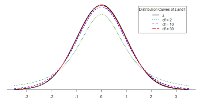
Figure \(\PageIndex{1}\) shows four curves: a normal distribution curve labeled \(z\), and three t-distribution curves for 2, 10, and 30 degrees of freedom. Two things should stand out: First, for lower degrees of freedom (e.g. 2), the tails of the distribution are much fatter, meaning the a larger proportion of the area under the curve falls in the tail. This means that we will have to go farther out into the tail to cut off the portion corresponding to 5% or \(α\) = 0.05, which will in turn lead to higher critical values. Second, as the degrees of freedom increase, we get closer and closer to the \(z\) curve. Even the distribution with \(df\) = 30, corresponding to a sample size of just 31 people, is nearly indistinguishable from \(z\). In fact, a \(t\)-distribution with infinite degrees of freedom (theoretically, of course) is exactly the standard normal distribution. Even though these curves are very close, it is still important to use the correct table and critical values, because small differences can add up quickly.
* Sometimes you'll see the one-sample t-test formula look like the following:
\[ t = \dfrac{(\bar{X}-\mu)}{s_{\bar{X}}} \nonumber \]
The \( s_{\bar{X}} \) means the same as \({s / \sqrt{n}} \), so let's just learn one formula and not get confused with something that looks like it might be a standard deviation but is not.
Contributors and Attributions
Foster et al. (University of Missouri-St. Louis, Rice University, & University of Houston, Downtown Campus)