11.4: Practice with Job Applicants

Let's practice our 4-step process using the ANOVA Summary Table to complete the calculations, but the Sum of Squares will be provided in this first example.

Scenario

Our data come from three groups of 10 people each, all of whom applied for a single job opening: those with no college degree, those with a college degree that is not related to the job opening, and those with a college degree from a relevant field. We want to know if we can use this group membership to account for our observed variability in their scores on a test related to the job that they applied for, and, by doing so, see if there is a difference between our three group means.  

To help understand what's going on in this scenario, let's answer some questions:

Exercise \(\PageIndex{1}\)

Answer the following questions to understand the variables and groups that we are working with.  

1. Who is the sample?  
2. Who do might be the population?   
3. What is the IV (groups being compared)?         
4. What is the DV (quantitative variable being measured)?

Answer

1. The sample is the 30 people with different degrees (or no degree)?  
2. The population might be any job applicant? 
3. The IV can be called "Degree," with the levels being:
   1. None,
   2. Related to job
   3. Unrelated to job
4. The DV is the score on the test.

Identifying the IV levels and DV helps when constructing your hypotheses.

Step 1: State the Hypotheses

Our hypotheses are concerned with the average score on the test for each of the groups based on education level, so you get to decide which groups you think will have a higher score, which groups will earn a lower average score, and which groups will have scores that are similar.

Exercise \(\PageIndex{2}\)

Determine the research hypothesis in words and symbols.  You can fill in the following underlined spot with the symbols for greater than (>), less than (<), or equal signs.  Just remember, at least one pair of means must be predicted to be different from each other.  

Symbols:

• \( \overline{X}_{N} \) _____ \( \overline{X}_{R} \)
• \( \overline{X}_{N} \) _____ \(\overline{X}_{U} \)
• \( \overline{X}_{R} \) _____ \(\overline{X}_{U} \)      

Answer

Here's a reasonable research hypothesis.  However, without the group means to guide us, your research hypothesis might be slightly different.  Just remember, at least one pair of means must be predicted to be different from each other.

• Research Hypothesis:    Those with No Degree will have a lower average test score than those with a Related Degree, but will have a similar average test score to those with an unrelated degree.  The average test score for those with a Related Degree will also have a higher average test score compared to those with an Unrelated Degree.
• Symbols:
  • \( \overline{X}_{N} < \overline{X}_{R} \)
  • \( \overline{X}_{N} = \overline{X}_{U} \)
  • \( \overline{X}_{R} > \overline{X}_{U} \)   

What about the null hypothesis?

Exercise \(\PageIndex{3}\)

State the null hypothesis in words and symbols.  

Answer

• Null Hypothesis:  The average test score will be similar for each group; the degree does not affect the hiring rate.
• Symbols:    \( \overline{X}_{N} = \overline{X}_{U} = \overline{X}_{R} \)

Step 2: Find the Critical Values

Our test statistic for ANOVA, as we saw above, is \(F\). Because we are using a new test statistic, we will get a new table: the \(F\) distribution table shown in the next section.  

There are now two degrees of freedom we must use to find our critical value: Numerator and Denominator. These correspond to the numerator and denominator of our test statistic, which, if you look at the ANOVA table presented earlier, are our Between Groups and Within Groups rows, respectively. The \(df_B\) is the Degrees of Freedom: for the Numerator because it is the degrees of freedom value used to calculate the Mean Square for the Between Groups source, which in turn was the numerator of our \(F\) statistic. Likewise, the \(df_W\) is the Degrees of Freedome for the Denominator because it is the degrees of freedom value used to calculate the Mean Square for the Within Groups (sometimes called Error) source, which was our denominator for \(F\).

The formula for \(df_B\) is \(k – 1\), and remember that k is the number of groups we are assessing. In this example, \(k = 3\) so our \(df_B\) = 2. This tells us that we will use the fourth column, the one labeled 2, to find our critical value. To find the proper row, we calculate the \(df_W\), which was \(N – k\). The original prompt told us that we have “three groups of 10 people each,” so our total sample size is 30. This makes our value for \(df_W\) = 27.  If we follow the fourth column down to the row for \(df_W\) = 27, then find the middle row for \(p\) = 0.05, we see that our critical value is 3.35. We use this critical value the same way as we did before: it is our criterion against which we will compare our calculated test statistic to determine statistical significance.

Step 3: Calculate the Test Statistic

Now that we have our hypotheses and the criterion we will use to test them, we can calculate our test statistic. To do this, we will fill in the ANOVA table. We will use the Sum of Squares values that we are provided in Table \(\PageIndex{1}\).

Table \(\PageIndex{1}\): ANOVA Summary Table

Source	\(SS\)	\(df\)	\(MS\)	\(F\)
Between	8246
Within	3020
Total	11266

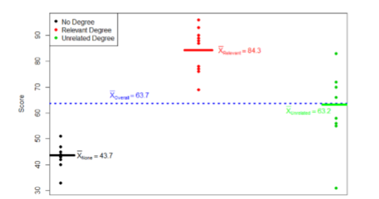
These may seem like random numbers, but remember that they are based on the distances between the groups themselves and within each group. Figure \(\PageIndex{2}\) shows the plot of the data with the group means and total mean included. If we wanted to, we could use this information, combined with our earlier information that each group has 10 people, to calculate the Between Groups Sum of Squares by hand. However, doing so would take some time, and without the specific values of the data points, we would not be able to calculate our Within Groups Sum of Squares, so we are just trusting that these values are the correct ones.

Figure \(\PageIndex{2}\): Means (CC-BY-NC-SA Foster et al. from An Introduction to Psychological Statistics)

Example \(\PageIndex{1}\)

Using the information provided in the scenario and Table \(\PageIndex{1}\), fill in the rest of the ANOVA Summary Table in Table \(\PageIndex{2}\)

Table \(\PageIndex{2}\): ANOVA Summary Table

Source	\(SS\)	\(df\)	\(MS\)	\(F\)
Between	8246
Within	3020
Total	11266

Solution

Using the formulas that we learned about earlier, we can complete Table \(\PageIndex{3}\):

Table \(\PageIndex{3}\)- ANOVA Summary Table with Formulas

Source	\(SS\)	\(df\)	\(MS\)	\(F\)
Between Groups	8246	\(k-1\) = 3 - 1 = 2	\(\frac{S S_{B}}{d f_{B}} = \frac{8246}{2} = 4123.00\)	\(\frac{MS_{B}}{MS_{W}} = \frac{4123.00}{11.85} = 36.86\)
Within Groups (Error)	3020	\(N-k\) = 30 - 3 = 27	\(\frac{S S_{W}}{d f_{W}} = \frac{3020}{27} = 11.85\)	N/A
Total	11266	\(N-1\) = 30 - 1 = 29	N/A	N/A

We leave those three empty cells blank; no information is needed from them. So, that leaves us with the final table looking like Table \(\PageIndex{4}\) showing calculated F-score of 36.86.

Table \(\PageIndex{4}\)- Completed ANOVA Summary Table

Source	\(SS\)	\(df\)	\(MS\)	\(F\)
Between Groups	8246	2	4123.00	36.86
Within Groups (Error)	3020	27	11.85	leave blank
Total	11266	29	leave blank	leave blank

 

We can move on to comparing our calculated value to the critical value in step 4.  

Step 4: Make the Decision

Our calculated test statistic was found to be \(F_{calc} = 36.86\) and our critical value was found to be \(F_{crit} = 3.35\). Our calculated statistic is larger than our critical value, so we can reject the null hypothesis.

Critical \(<\) Calculated \(=\) Reject null \(=\) At least one mean is different from at least one other mean. \(=\) p<.05

Critical \(>\) Calculated \(=\) Retain null \(=\)  All of the means are similar. \(=\)  p>.05

Based on our three groups of 10 people, we can conclude that average job test scores are statistically significantly different based on education level, \(F(2,27)=36.86,p<.05\).  Notice that when we report \(F\), we include both degrees of freedom. We always report the numerator then the denominator, separated by a comma.

Because we were only testing for any difference, we cannot yet conclude which groups are different from the others or if our research hypothesis was supported, partially supported, or not supported. We will learn about pairwise comparisons next to answer these last questions!

Contributors and Attributions

• Foster et al. (University of Missouri-St. Louis, Rice University, & University of Houston, Downtown Campus)

• Dr. MO (Taft College)