8.4.1: Descriptive and Inferential Calculations and Conclusion Example

Last updated
Save as PDF

Page ID: 18051

\( \newcommand{\vecs}[1]{\overset { \scriptstyle \rightharpoonup} {\mathbf{#1}} } \) \( \newcommand{\vecd}[1]{\overset{-\!-\!\rightharpoonup}{\vphantom{a}\smash {#1}}} \)\(\newcommand{\id}{\mathrm{id}}\) \( \newcommand{\Span}{\mathrm{span}}\) \( \newcommand{\kernel}{\mathrm{null}\,}\) \( \newcommand{\range}{\mathrm{range}\,}\) \( \newcommand{\RealPart}{\mathrm{Re}}\) \( \newcommand{\ImaginaryPart}{\mathrm{Im}}\) \( \newcommand{\Argument}{\mathrm{Arg}}\) \( \newcommand{\norm}[1]{\| #1 \|}\) \( \newcommand{\inner}[2]{\langle #1, #2 \rangle}\) \( \newcommand{\Span}{\mathrm{span}}\) \(\newcommand{\id}{\mathrm{id}}\) \( \newcommand{\Span}{\mathrm{span}}\) \( \newcommand{\kernel}{\mathrm{null}\,}\) \( \newcommand{\range}{\mathrm{range}\,}\) \( \newcommand{\RealPart}{\mathrm{Re}}\) \( \newcommand{\ImaginaryPart}{\mathrm{Im}}\) \( \newcommand{\Argument}{\mathrm{Arg}}\) \( \newcommand{\norm}[1]{\| #1 \|}\) \( \newcommand{\inner}[2]{\langle #1, #2 \rangle}\) \( \newcommand{\Span}{\mathrm{span}}\)\(\newcommand{\AA}{\unicode[.8,0]{x212B}}\)

Let's use data that Dr. MO's student research group collected on growth mindset from students at a community college. We'll start by interpreting the descriptive statistics and graph of the sample from the output of statistical software, then go step-by-step through a one-sample t-test.

Here we go!

Scenario

Students in Dr. MO's research group conducted an experiment in which several faculty members used videos, readings, and in-class discussion to try to improve the growth mindset (see 7.1) of their students. We will start by looking at the pretest scores of all 126 community college students in this study. In other words, we are looking at the students' scores on an assessment of their mindset before they had learned anything about growth mindset. The survey score could be from 0 points (totally fixed mindset) to 60 points (totally growth mindset), with any score above 33 points having more growth mindset beliefs.

Let's describe what we know already!

Exercise \(\PageIndex{1}\)

1. Based on the scenario, who is the sample? Your answer should include the number of people in the sample.

2. Based on this sample, who could be the population? Why?

3. What is the DV (effect)? In other words, what was the outcome that was measured?

Answer

1. 126 community college students

2. Any reasonable population based on the sample, but probably community college students in the U.S.

3. Scores on the mindset assessment.

Now, let's learn more about this sample, and interpret what these descriptive statistics can show us!

Descriptive Statistics

Measures of Central Tendency

The measures of central tendency are shown in Table \(\PageIndex{1}\).

Table \(\PageIndex{1}\)- Measures of Central Tendency for Mindset Pretest
Measure of Central Tendency	Result
N	126
Mean	42.06
Median	41.00
Mode	39

What can we learn from these measures of central tendency?

Exercise \(\PageIndex{2}\)

Knowing the mean, median, and mode, what could be the “center” of this distribution of mindset scores? In other words, what one number might represent a typical score? Why do you think that?

Answer: The mean (\( \bar{X} =42.06 points\)) and median (Md = 41 points)) are relatively close, suggesting that the "center" of this distribution is 41 or 42 points. However, because the mode is lower (Mode = 39 points), the center is probably closer to that lower number of 41 points.

As you know, measures of central tendency don't tell the whole story about a distribution. Let's look at varibility next.

Measure of Variability

The main measure of variability that we look at is standard deviation. The standard deviation of this sample of mindset scores is 6.65 points. We can also look at the highest and lowest scores to see the range. The lowest mindset score in this sample was 28 points, and the highest score was the maximum of 60 points. What can this tell us about the distribution?

Exercise \(\PageIndex{3}\)

Based on the mean and standard deviation only, do you think that the distribution of mindset scores will be tall and narrow, short and wide, or a medium bell-curve? Why?

Answer: I think that a standard deviation of 6.65 is medium, so I think that the distribution will be a bell-shaped curve. However, since no once scored below 28 points, maybe it's negatively skewed (a tail pointing to the left with the bulk of scores to the right.

I literally was just guessing in Exercise \(\PageIndex{3}\). Let's look at the actual frequencies to see if I guessed correctly!

Frequency

Table \(\PageIndex{2}\) is a frequency table for this sample's mindset scores, and Figure \(\PageIndex{1}\) shows the same information in a line graph.

Table \(\PageIndex{2}\)- Frequency of Mindset Scores
X (Mindset Score)	Frequency
28	1
30	1
31	2
32	3
33	6
34	2
35	3
36	7
37	9
38	6
39	12
40	7
41	5
42	7
43	8
44	3
45	8
46	3
47	7
48	5
49	5
51	4
52	2
53	2
54	3
55	1
56	1
57	1
60	2

And Figure \(\PageIndex{1}\):

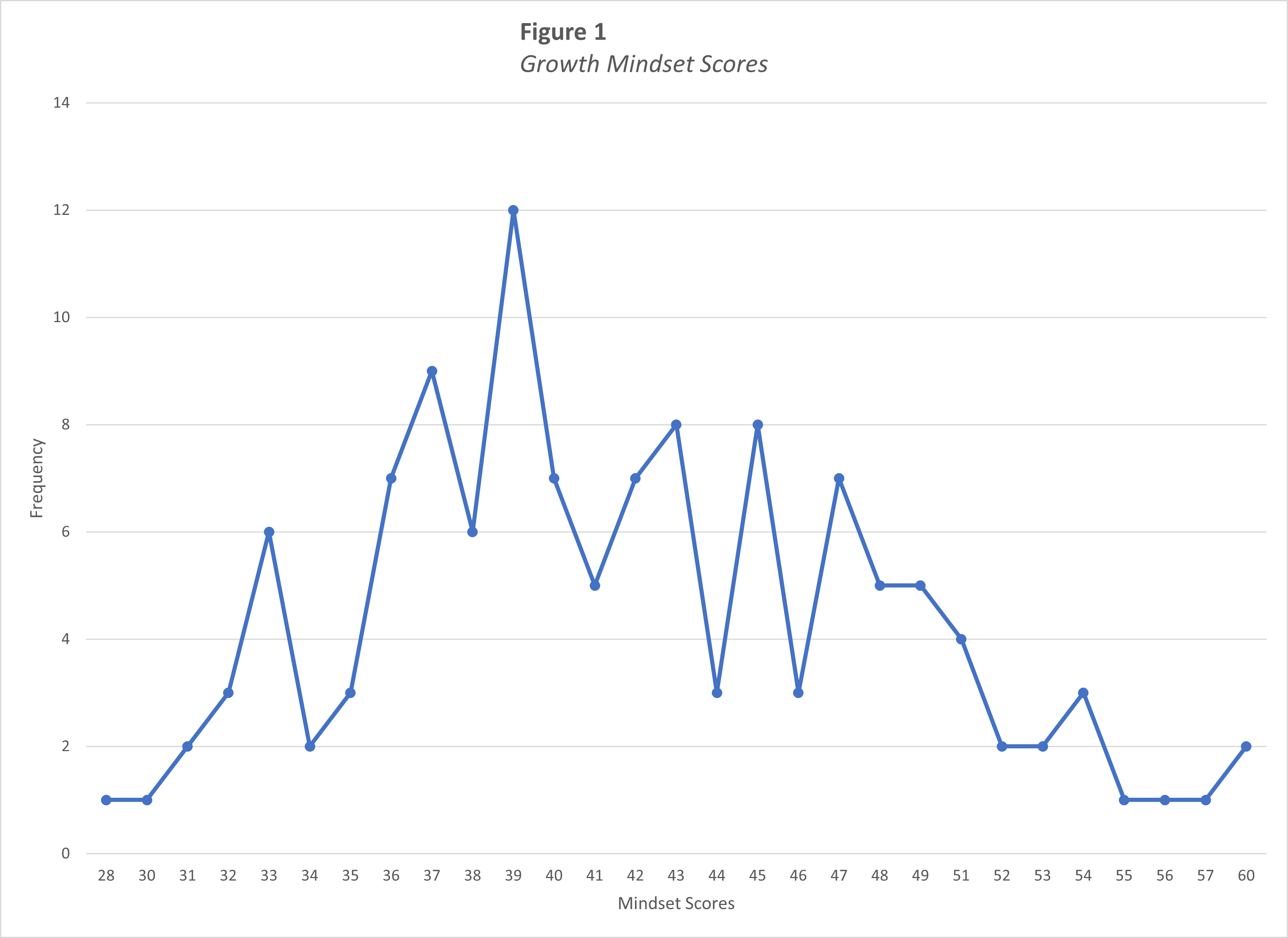
Line graph showing frequency of mindset scores from the sample. — Figure \(\PageIndex{1}\): Frequency Line Graph of Mindset Scores. (CC-BY-NC-SA; Michelle Oja)

Let's start unpacking Figure \(\PageIndex{1}\).

Exercise \(\PageIndex{4}\)

What kind of graph is Figure \(\PageIndex{1}\)?
What does the x-axis measure in Figure \(\PageIndex{1}\)?
What does the y-axis measure in Figure \(\PageIndex{1}\)?
Is Figure \(\PageIndex{1}\) skewed? If so positively or negatively? If not, is the graph tall/narrow, medium/normal, or wide/flat?
What do you notice from Figure \(\PageIndex{1}\)? What pops out to you?
What does Figure \(\PageIndex{1}\) make you wonder about?
What is a catchy headline for Figure \(\PageIndex{1}\)?
How could you summarize the info in Figure \(\PageIndex{1}\) into one sentence?
Who might want to know the information in Figure \(\PageIndex{1}\)?

Answer

What kind of graph is Figure \(\PageIndex{1}\)?
1. Figure \(\PageIndex{1}\) is a line graph showing frequencies.
What does the x-axis measure in Figure \(\PageIndex{1}\)?
1. The x-axis measures mindset scores.
What does the y-axis measure in Figure \(\PageIndex{1}\)?
1. The y-axis measures frequencies of each mindset score.
Is Figure \(\PageIndex{1}\) skewed? If so positively or negatively? If not, is the graph tall/narrow, medium/normal, or wide/flat?
1. Although the mode isn't quite in the center, I would say that this frequency distribution is not skewed. It seems to be a medium normal curve (not tall/narrow or wide/flat).
What do you notice from Figure \(\PageIndex{1}\)? What pops out to you?
1. I was actually surprised by how symmetrical the distribution was! I also noticed that no one scored below 28 points, even though someone could score all the way down to zero points on this mindset assessment.
What does Figure \(\PageIndex{1}\) make you wonder about?
1. This makes me wonder why no one scored low; the cut-off for having a fixed mindset is 33 points, so it's surprising that few students in this sample have a fixed mindset.
What is a catchy headline for Figure \(\PageIndex{1}\)?
1. Community College Students Start with Growth!
How could you summarize the info in Figure \(\PageIndex{1}\) into one sentence?
1. From this sample, I might infer that 90% of community college students hold growth mindset views.
Who might want to know the information in Figure \(\PageIndex{1}\)?
1. Definitely community college faculty and adminstrators, as well as researchers who want to learn about growth mindset or improve student performance.

Okay, now that we've looked at Figure \(\PageIndex{1}\) closely, let's think about it in relation to the measures of central tendencies.

Exercise \(\PageIndex{5}\)

First, look back at your answer about whether the distribution would be tall/narrow, flat/wide, or medium/bell-shaped. Were you correct? Reflect on what about this distribution of data made it easier or more difficult to predict the shape based on these descriptive statistics.

Second, knowing the mean, median, mode, standard deviation, and what the distribution looks like, do you think that community college students tend to have fixed mindsets or growth mindsets?

Answer

First, yes, I believe that I estimated correctly. I said that the distribution should be medium and bell-shaped, and I think that it is. I think it was easier to correctly estimate the shape because the mean and median were so close. But that lower mode was a little confusing!

Second, knowing the mean, median, mode, standard deviation, and what the distribution looks like, think that community college students tend to have growth mindsets. The measures of central tendency are all above the cut-off of 33 points for a fixed mindset, and the graph shows that only a few students had fixed mindsets. Also, the standard deviation wasn't too high, which suggests that there are no outliers (extreme scores), which the graph confirms.

You might wonder why we went through all of this. The answers to these questions will be what you use to for a future paper analyzing a data set. Plus, now you know more about growth mindset of community college students!

Note

Now that you have the full data set, you are encouraged to calculate the mean, median, mode, and standard deviation yourself, and create your own graph as a refresher! (If you do, note that the data is in a frequency table, it is not a list of all of the scores individually...)

But this chapter isn't about growth mindset or descriptive statistics. This chapter is about one-sample t-tests, so let's get to that!

Null Hypothesis Significance Testing Steps

Step 1: State the Hypotheses

Let's start with a research hypothesis.

When the student researchers first started on this research project, we were very surprised by how high the mindset scores start out. Other research suggests that the cut-off of 33 points is a good estimate of the general population's mindset scores. This leads to:

Research Hypothesis: Community college students' average mindset scores are higher than the general population's mindset scores.
Symbols: \( \bar{X} > \mu \)

Exercise \(\PageIndex{6}\)

Based on the research hypothesis, what is the null hypothesis? Write it out in words, then in symbols.

Answer

Null Hypothesis: Community college students' average mindset scores as similar to the general population's mindset scores.
Symbols: \( \bar{X} = \mu \)

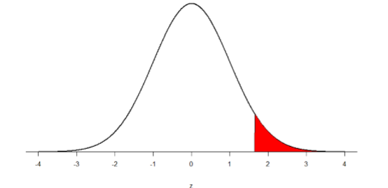
Step 2: Find the Critical Values

You know that the most common level of significance is \(α\) = 0.05, so you keep that the same. Using the table of critical values for the t-distribution, what critical value do we use?

Example \(\PageIndex{1}\)

First, what Degrees of Freedom would you use?

Second, what is the critical t-score?

Solution

First, \(df = N - 1\), so:

\[ 126 - 1 = 125 \nonumber \]

Second, for df=126, we use df=100 from the table (because it is both the closest whether you round up or down). The critical t-score for df=100 is 1.660.

To keep track of the directionality of the test and rejection region, you draw out your distribution:

Standard normal curve showing extreme right shaded to indicate the Rejection Region. — Figure \(\PageIndex{2}\): Rejection region (CC-BY-NC-SA Foster et al. from An Introduction to Psychological Statistics)

Step 3: Calculate the Test Statistic

Okay, you have everything you need to calculate the one-sample t-test! To make sure it's all in one place, Table \(\PageIndex{3}\) puts all of the numbers in one place. This might be a good practice everytime that you conduct a statistical analysis...

Table \(\PageIndex{3}\)- Necessary Information for One-Sample t-test
Necessary Information	Numbers
N	126
Mean of the Sample	42.06
Std. Deviation	6.65
Mean of the Population	33.00

\[t=\cfrac{(\bar{X}-\mu)}{\left(\cfrac{s} {\sqrt{n}}\right)} = \cfrac{(42.06 - 33)}{\left(\cfrac{6.65} {\sqrt{126}}\right)} = \cfrac{(9.06)}{\left(\cfrac{6.65} {11.22}\right)} = \dfrac{9.06}{0.59} = 15.29 \nonumber \]

Step 4: Make the Decision

You compare your calculated \(t\)-statistic (\(t\) = 15.29), to the critical value, \(t_crit\) = 1.6600, and find that the calculated score is bigger than the critical value.

Remember:

Critical < |Calculated| = Reject null = \( \bar{X} \neq \mu \) = p<.05

Critical > |Calculated| = Retain null = \( \bar{X}=\mu \) = p>.05

So, we reject the null hypothesis, and write up our conclusion.

Write-Up

Remember the four components that should be in a complete conclusion?

Exercise \(\PageIndex{7}\)

What should your write-up of the t-test results look like?

Answer: I hypothesized that the sample's mindset scores (\( \bar{X} = 42.06 points \) would be higher than mindset scores of the population (\( \mu = 33 points \)). This research hypothesis was supported (t(125) = 15.29, p< 0.05); the sample of community college students did have higher mindset scores than the general population.

Cool, huh?!

Contributors and Attributions

Foster et al. (University of Missouri-St. Louis, Rice University, & University of Houston, Downtown Campus)
Dr. MO (Taft College)

X (Mindset Score)	Frequency
28	1
30	1
31	2
32	3
33	6
34	2
35	3
36	7
37	9
38	6
39	12
40	7
41	5
42	7
43	8
44	3
45	8
46	3
47	7
48	5
49	5
51	4
52	2
53	2
54	3
55	1
56	1
57	1
60	2

X (Mindset Score)	Frequency
28	1
30	1
31	2
32	3
33	6
34	2
35	3
36	7
37	9
38	6
39	12
40	7
41	5
42	7
43	8
44	3
45	8
46	3
47	7
48	5
49	5
51	4
52	2
53	2
54	3
55	1
56	1
57	1
60	2

X (Mindset Score)	Frequency
28	1
30	1
31	2
32	3
33	6
34	2
35	3
36	7
37	9
38	6
39	12
40	7
41	5
42	7
43	8
44	3
45	8
46	3
47	7
48	5
49	5
51	4
52	2
53	2
54	3
55	1
56	1
57	1
60	2