7.5.1: Critical Values

Okay, this whole chapter is full of complex theoretical ideas.  Critical values and null hypothesis significance testing is a TOUGH concept to get.  Here's another description of critical values, p-values, and significance.  Everyone learns differently, so hopefully this slightly different explanation will help understand the prior section.  

Hypotheses

We understand that we need a research hypothesis that predicts the relationship between two groups on an measured outcome (DV), and that each research hypothesis has a null hypothesis that says that there is no relationship between the two groups on the measured outcome (the means of the DV are similar).  If we reject the null hypothesis (which says that the means are similar), we are saying that the means are different; this may or may not be in the direction that we predicted in the research hypothesis so we may or may not support the research hypothesis.  If we retain (fail to reject) the null hypothesis, we are saying that the means are similar and then we cannot support the research hypothesis.  Got it?

But how do we decide again to retain or reject the null hypothesis?  We compare a calculated statistic (there are many, depending on your variables, that we'll cover for the rest of this textbook) to a critical value from a table.  The table uses probability (p-values) to tell us what calculated values are so extreme to be absolutely unlikely.  

Critical Regions and Critical Values

The critical region of any test corresponds to those values of the test statistic that would lead us to reject null hypothesis (which is why the critical region is also sometimes called the rejection region). How do we find this critical region? Well, let’s consider what we know:

• The test statistic should be very big or very small (extreme) in order to reject the null hypothesis.
• If α=.05 (α is "alpha," and is just another notation for probability; we'll talk about it more in the section on errors), the critical region must cover 5% of a Standard Normal Distribution.

It’s only important to make sure you understand this last point when you are dealing with non-directional hypotheses (which we will only do for Confidence Intervals). The critical region corresponds to those values of the test statistic for which we would reject the null hypothesis, and the Standard Normal Distribution describes the probability that we would obtain a particular value if the null hypothesis (that the means are similar) were actually true. Now, let’s suppose that we chose a critical region that covers 20% of the Standard Normal Distribution, and suppose that the null hypothesis is actually true. What would be the probability of incorrectly rejecting the null (saying that there is a difference between the means when there really isn't a difference)? The answer is 20%. And therefore, we would have built a test that had an α level of 0.2. If we want α=.05, the critical region only covers 5% of the Standard Normal Distribution.

Huh?  Let's draw that out.  Figure \(\PageIndex{1}\) shows the critical region associated with a non-directional hypothesis test (also called a "two-sided test" because the calculated value might be in either tail of the distribution). Figure \(\PageIndex{1}\) itself shows the sampling distribution of X (the scores we got).  The grey bars correspond to those values for which we would retain the null hypothesis. The blue (dark) bars show the critical region: those values for which we would reject the null. In this example, the research hypothesis was non-directional, so the critical region covers both tails of the distribution. To ensure an α level of .05, we need to ensure that each of the two regions encompasses 2.5% of the sampling distribution.

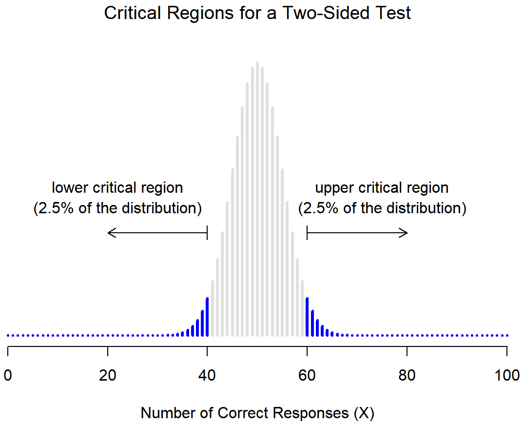
Figure \(\PageIndex{1}\)- Example of Critical Regions for a Non-Directional Research Hypothesis (CC-BY-SA- Danielle Navarro from Learning Statistics with R)

Our critical region consists of the most extreme values, known as the tails of the distribution. 

At this point, our hypothesis test is essentially complete: (1) we choose an α level (e.g., α=.05, (2) come up with some test statistic (more on this step later) that does a good job (in some meaningful sense) of comparing the null hypothesis to the research hypothesis, (3) calculate the critical region that produces an appropriate α level, and then (4)  calculate the value of the test statistic for the real data and then compare it to the critical values to make our decision. If we reject the null hypothesis, we say that the test has produced a significant result.

A note on statistical “significance”

Like other occult techniques of divination, the statistical method has a private jargon deliberately contrived to obscure its methods from non-practitioners.

– Attributed to G. O. Ashley*

A very brief digression is in order at this point, regarding the word “significant”. The concept of statistical significance is actually a very simple one, but has a very unfortunate name. If the data allow us to reject the null hypothesis, we say that “the result is statistically significant”, which is often shortened to “the result is significant”. This terminology is rather old, and dates back to a time when “significant” just meant something like “indicated”, rather than its modern meaning, which is much closer to “important”. As a result, a lot of modern readers get very confused when they start learning statistics, because they think that a “significant result” must be an important one. It doesn’t mean that at all. All that “statistically significant” means is that the data allowed us to reject a null hypothesis. Whether or not the result is actually important in the real world is a very different question, and depends on all sorts of other things.

Directional and Non-Directional Hypotheses

There’s one more thing to point out about the hypothesis test that we’ve just constructed. In statistical language, this is an example of a non-directional hypothesis, also known as a two-sided test. It’s called this because the alternative hypothesis covers the area on both “sides” of the null hypothesis, and as a consequence the critical region of the test covers both tails of the sampling distribution (2.5% on either side if α=.05), as illustrated earlier in Figure \(\PageIndex{1}\).

However, that’s not the only possibility, and not the situation that we'll be using with our directional research hypotheses (the ones that predict which group will have a higher mean).  A directional research hypothesis would only cover the possibility that p>.5, and as a consequence the null hypothesis now becomes p≤.5.  When this happens, we have what’s called a one-sided test, and when this happens the critical region only covers one tail of the sampling distribution. This is illustrated in Figure \(\PageIndex{2}\).   In this case, we would only reject the null hypothesis for large values of of our test statistic (values that are more extreme but only in one direction). As a consequence, the critical region only covers the upper tail of the sampling distribution; specifically the upper 5% of the distribution. Contrast this to the two-sided version earlier in Figure \(\PageIndex{1}\).

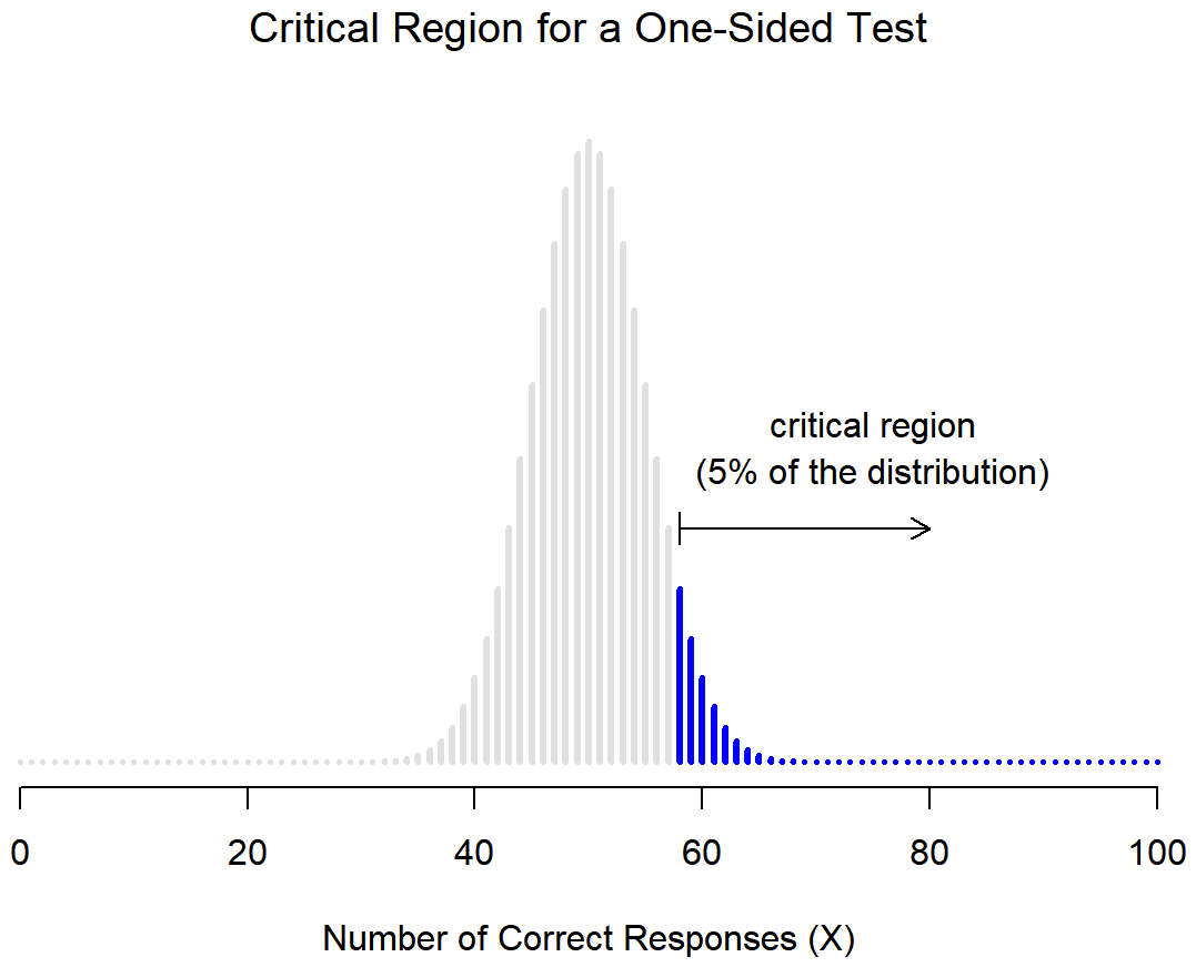
Figure \(\PageIndex{2}\)- Critical Region for Directional Research Hypotheses (CC-BY-SA- Danielle Navarro from Learning Statistics with R)

Clear as mud?  Let's try one more way to describe how research hypotheses, null hypotheses, p-values, and null hypothesis significance testing work.

References

*The internet seems fairly convinced that Ashley said this, though I can’t for the life of me find anyone willing to give a source for the claim.

Contributors and Attributions

• Danielle Navarro (University of New South Wales)

• Dr. MO (Taft College)