
3.5: Introduction to Measures of Variability
- Page ID
- 17319

Variability refers to how “spread out” a group of scores is. To see what we mean by spread out, consider graphs in Figure \(\PageIndex{1}\). These graphs represent the GPA and the hours that the student studied (the GPA_Study_Hours file from www.OpenIntro.org/data website). You can see that the distributions are quite different. Specifically, the scores on Figure \(\PageIndex{1}\) are more densely packed and those on Figure \(\PageIndex{2}\) are more spread out. The differences among students in the hours that they studies were much greater than the differences among the same students on their GPA. These histograms show that some scores are closer to the mean than other scores, and that some distributions have more scores that are closer to the mean and other distributions have scores that tend to be farther from the mean. Sometimes, knowing one, or all, of the measures of central tendency is not enough.
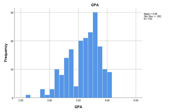
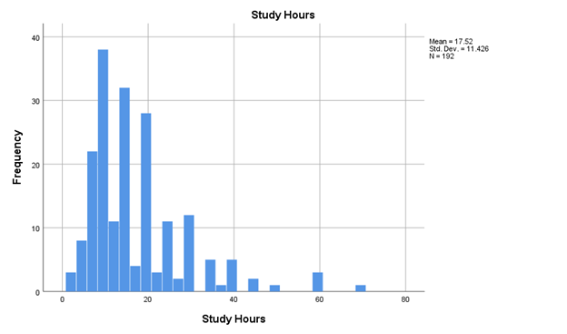
Figure \(\PageIndex{3}\) shows sets of two normal distributions. Notice that some distributions are tall and narrow, and some are wider and flatter. The tall and narrow distribution has small variability between each score and the mean, and the wide and flat distribution has more variability between each score and the mean. The mean is a better description of the distribution of the data when it is tall and narrow since most scores aren't that different from the mean.
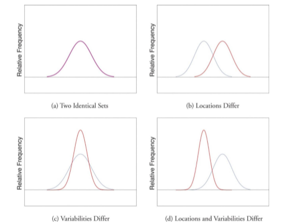
Figure \(\PageIndex{3}\): Differences between two datasets. (CC-BY-NC-SA Foster et al. from An Introduction to Psychological Statistics)
The terms variability, spread, and dispersion are synonyms, and refer to how spread out a distribution is. Just as in the section on central tendency where we discussed measures of the center of a distribution of scores, in this section we will discuss measures of the variability of a distribution. We will focus on two frequently used measures of variability: range and standard deviation. We'll start with range now, then move on to standard deviation next.
Range
The range is the simplest measure of variability to calculate, and one you have probably encountered many times in your life. The range is simply the highest score minus the lowest score. Let’s take a few examples. What is the range of the following group of numbers: 10, 2, 5, 6, 7, 3, 4? Well, the highest number is 10, and the lowest number is 2, so 10 - 2 = 8. The range is 8. Let’s take another example. Here’s a dataset with 10 numbers: 99, 45, 23, 67, 45, 91, 82, 78, 62, 51. What is the range? The highest number is 99 and the lowest number is 23, so 99 - 23 equals 76; the range is 76. Now consider the two quizzes shown in Figure \(\PageIndex{1}\) and Figure \(\PageIndex{2}\). On Quiz 1, the lowest score is 5 and the highest score is 9. Therefore, the range is 4. The range on Quiz 2 was larger: the lowest score was 4 and the highest score was 10. Therefore the range is 6.
The problem with using range is that it is extremely sensitive to outliers, and one number far away from the rest of the data will greatly alter the value of the range. For example, in the set of numbers 1, 3, 4, 4, 5, 8, and 9, the range is 8 (9 – 1).
However, if we add a single person whose score is nowhere close to the rest of the scores, say, 20, the range more than doubles from 8 to 19.
Contributors
Foster et al. (University of Missouri-St. Louis, Rice University, & University of Houston, Downtown Campus)