2.10: Graphing Quantitative Data- Boxplots

You might think that you've never seen a box plot, but you probably have seen something similar.   

An alternative to line graphs and histograms is a boxplot, sometimes called a “box and whiskers” plot. Like line graphs and histograms, they’re best suited to quantitative data (interval or ratio scale of measurement). The idea behind a boxplot is to provide a simple visual depiction of the score in the exact middle (median), the where about each fourth (quartile) of the scores are, and the range of the data. And because boxplots do so in a fairly compact and intuitive way, they have become a very popular statistical graphic. When you look at this plot, this is how you should interpret it: the thick line in the middle of the box is the median; the box itself spans the range from the 25th percentile to the 75th percentile; and the “whiskers” cover the full range from the minimum value to the maximum value. This is summarized in the annotated plot in Figure \(\PageIndex{1}\).

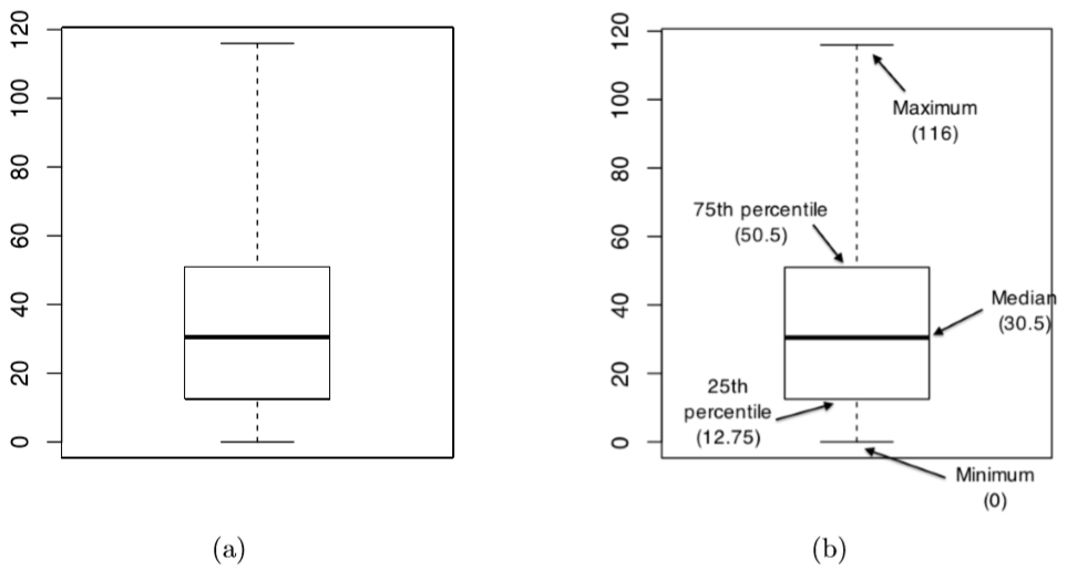
Figure \(\PageIndex{1}\)- A basic boxplot (panel a), plus the same plot with annotations added to explain what aspect of the data set each part of the boxplot corresponds to (panel b).  (CC-BY-SA- Danielle Navarro from Learning Statistics with R)

In most applications, the “whiskers” don’t cover the full range from minimum to maximum. Instead, they actually go out to the most extreme data point that doesn’t exceed a certain bound. By default, this value is 1.5 times the interquartile range (you don't have to know what all of that means). Any observation whose value falls outside this range is plotted as a circle instead of being covered by the whiskers, and is commonly referred to as an outlier. Because the boxplot automatically separates out those observations that lie outside a certain range, people often use them as an informal method for detecting outliers: observations that are “suspiciously” distant from the rest of the data.

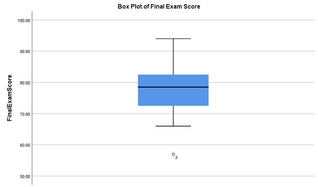
Our Final Exam Score data provides just such an example, as shown in Figure \(\PageIndex{2}\), a boxplot created with SPSS software (standard spreadsheet software generally does not include boxplot options).  If you look closely, there's a little circle under the bottom whisker with a "3" next to it.  This is showing that three scores were below the range of the whiskers.  These three scores can be considered outliers.  If you go back to Figure 2.2.2, you can easily see what those three scores are (57, 66, 69).

Figure \(\PageIndex{2}\)- Boxplot of Frequency of Final Exam Scores. (Copyright CC-SA, chart by Dr. MO via data provided by OpenIntro.org )

Box Plots Interpretation

Let's answer the same questions that we've been answering, over this same data set, but based on the boxplot graphic in Figure \(\PageIndex{2}\).

1. What kind of graph is Figure Figure \(\PageIndex{2}\)?
   1. This box plot.    
2. What does the x-axis measure in Figure \(\PageIndex{2}\)?
   1. There is no x-axis because there is only one group.  If there were more groups, each would have its own box and the name of the group would be labeled on the x-axis. 
3. What does the y-axis measure in Figure \(\PageIndex{2}\)?
   1. The y-axis is the axis that goes up and down.  In Figure \(\PageIndex{2}\),the y-axis shows how many students earned different scores on the Final Exam by the size and location of the square in the middle.  The “whiskers” or bars show information about the expected variation.  You can also see a circle under the 60.00 line, with the number 3 next to it; this shows that 3 students scored that extreme, which is outside of what is expected. 
4. Is Figure Figure \(\PageIndex{2}\)?  If so positively or negatively?  If not, is the graph tall/narrow, medium/normal, or wide/flat? 
   1. This is sort of a trick question.  Skew is not shown in a box plot in the same way that it is shown in a line graph or histogram.  However, you can see that the box in the middle is not centered evenly between the whiskers; the top whisker is longer than the bottom whisker.  This shows that the bulk of scores fall within the box, but that there are some that go higher and lower, and the circle shows that there are three scores that are really low. 
5. What do you notice from Figure \(\PageIndex{2}\)?  What pops out to you?
   1. Those three scores at the bottom jump out at me!  Plus, the fact that the top whisker doesn’t go all the way to 100 suggests that no one scored that high. 
6. What does Figure \(\PageIndex{2}\) make you wonder about?
   1. This box plot makes me wonder about those three students outside of the whiskers more than the other charts did.  
7. What is a catchy headline for Figure \(\PageIndex{2}\)?
   1. Chances Are You’ll Be One of the 85% [Because 17 out of 20 students earned a passing grade on the Final Exam; 17/20 = .85 x 100 = 85%]
8. How could you summarize the info in Figure \(\PageIndex{2}\) into one sentence?
   1. The class did really well on the Final Exam, although three students did not pass.
9. Who might want to know the information in Figure \(\PageIndex{2}\)?
   1. I still am guessing that students who are going to take this class from this professor might be interested.  College administrators might also want to know so that they can see that most students are passing their classes.

That's it on boxplots!  Let's move on to the last kind of graph that will be discussed, scatterplots!

Contributors and Attributions

• Danielle Navarro (University of New South Wales)

• Dr. MO (Taft College)