
9.1.1: Another way to introduce independent sample t-tests...
- Page ID
- 22089

Although the one sample t-test has its uses, it’s not the most typical example of a t-test. A much more common situation arises when you’ve got two different groups of observations. In psychology, this tends to correspond to two different groups of participants, where each group corresponds to a different condition in your study. For each person in the study, you measure some outcome variable of interest (DV), and the research question that you’re asking is whether or not the two groups have the same population mean (each group is considered a level of the IV). This is the situation that the independent samples t-test is designed for.
Example
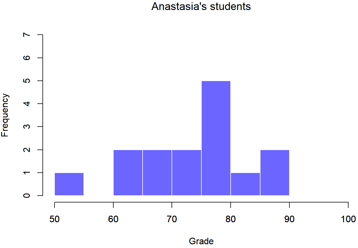
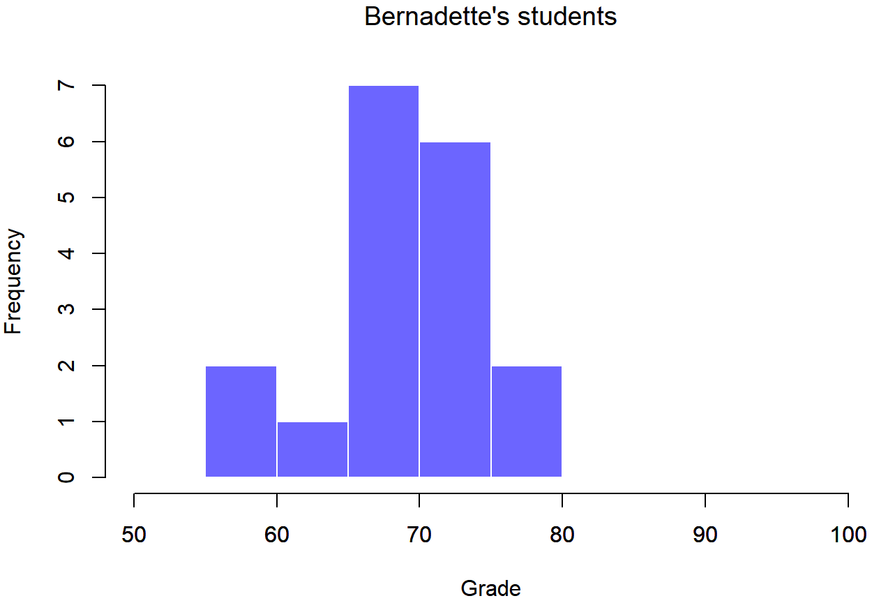
Suppose we have 33 students taking Dr Harpo’s statistics lectures, and Dr Harpo doesn’t grade to a curve. Actually, Dr Harpo’s grading is a bit of a mystery, so we don’t really know anything about what the average grade is for the class as a whole (no population mean). There are two tutors for the class, Anastasia and Bernadette. There are NA=15 students in Anastasia’s tutorials, and NB=18 in Bernadette’s tutorials. The research question I’m interested in is whether Anastasia or Bernadette is a better tutor, or if it doesn’t make much of a difference. Dr Harpo emails Dr. Navarro the course grades, and Dr. Navarro finds the mean and standard deviation (shown in Table \(\PageIndex{1}\)).
| Mean | Standard Deviation | N | |
|---|---|---|---|
| Bernadette’s students | 69.06 | 5.77 | 18 |
| Anastasia’s students | 74.53 | 9.00 | 15 |
To give you a more detailed sense of what’s going on here, Dr. Navarro plotted histograms showing the distribution of grades for both tutors (Figure \(\PageIndex{1}\) and Figure \(\PageIndex{2}\)). Inspection of these histograms suggests that the students in Anastasia’s class may be getting slightly better grades on average, though they also seem a little more variable.
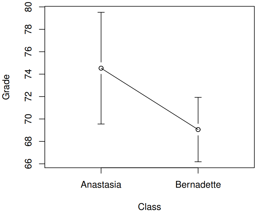
Here is a simpler plot showing the means and corresponding confidence intervals for both groups of students (Figure \(\PageIndex{3}\)). On the basis of visual inspection, it does look like there’s a real difference between the groups, though it’s hard to say for sure.
This is where an independent sample t-test would come in! We aren't comparing a sample's mean score to a population's mean score like we did last chapter with the one-sample t-test. Instead, we are comparing the means of two groups to see if they are from the same population (in other words, to see if the two groups are similar).
Independent Sample t-test
Let's talk about the Student t-test. The goal is to determine whether two “independent samples” of data are drawn from populations with the same mean (the null hypothesis) or different means. When we say “independent” samples, what we really mean here is that there’s no special relationship between observations in the two samples. This probably doesn’t make a lot of sense right now, but it will be clearer when we come to talk about the paired samples t-test later on. For now, let’s just point out that if we have an experimental design where participants are randomly allocated to one of two groups, and we want to compare the two groups’ mean performance on some outcome measure, then an independent samples t-test (rather than a paired samples t-test) is what we’re after.
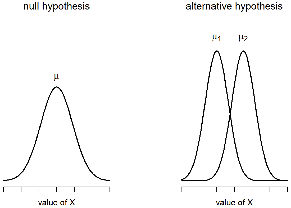
Okay, so let’s let μ1 denote the true population mean for group 1 (e.g., Anastasia’s students), and μ2 will be the true population mean for group 2 (e.g., Bernadette’s students), and as usual we’ll let \(\bar{X}_{1}\) and \(\bar{X}_{2}\) denote the observed sample means for both of these groups. Our null hypothesis states that the two population means are identical (μ1=μ2) and the alternative to this is that they are not (μ1≠μ2). Figure \(\PageIndex{4}\) shows this concept graphically. Notice that it is assumed that the population distributions are normal, and that, although the alternative hypothesis allows the group to have different means, it assumes they have the same standard deviation.
To construct a hypothesis test that handles this scenario, we start by noting that if the null hypothesis is true, then the difference between the population means is exactly zero, \(\mu_1 - \mu_2 = 0\) As a consequence, a diagnostic test statistic will be based on the difference between the two sample means. Because if the null hypothesis is true, then we’d expect
\(\bar{X}_{1}\) - \(\bar{X}_{2}\)
to be pretty close to zero. However, just like we saw with our one-sample t-tests, we have to be precise about exactly how close to zero this difference
\(\ t ={\bar{X}_1 - \bar{X}_2 \over SE}\)
We just need to figure out what this standard error estimate actually is. This is a bit trickier than was the case for either of the two tests we’ve looked at so far, so we need to go through it a lot more carefully to understand how it works. We will do that later when discussing the actual formula. For now, just recognize that you're using something like a standard deviation to divide everything by in order to create something like an average difference between the two groups.
Results
If we used statistical software to calculate this t-test, we'd get a statistical sentence of: t(31)=2.12, p<.05 This is telling you that the results for the calculated t-test was 2.12, that the degrees of freedom are 31, and that the probability is less than 5% that the groups are similar (that they are from the same popuolation). The degrees of freedom might look new. You can think of the degrees of freedom to be equal to the number of data points minus the number of constraints. In this case, we have N observations (N1 in sample 1, and N2 in sample 2), and 2 constraints (the sample means). So the total degrees of freedom for this test are \(N_1 + N_2 - 2\). These results tell you that the difference between the two groups is statistically significant (just barely), so we might write up the result using text like this:
The mean grade in Anastasia’s class was \(74.5\%\) (s=9.0), whereas the mean in Bernadette’s class was \(69.1\%\) (s=5.8). A Student’s independent samples t-test showed that this difference was significant (t(31)=2.12, p<.05), suggesting that a genuine difference in learning outcomes has occurred.
Positive and Negative t-scores
Before moving on to talk about the assumptions of the t-test, there’s one additional point I want to make about the use of t-tests in practice. The first one relates to the sign of the t-statistic (that is, whether it is a positive number or a negative one). One very common worry that students have when they start running their first t-test is that they often end up with negative values for the t-statistic, and don’t know how to interpret it. In fact, it’s not at all uncommon for two people working independently to end up with results that are almost identical, except that one person has a negative t values and the other one has a positive t value. This is perfectly okay: whenever this happens, what you’ll find is that the two versions are based on which sample mean you put as \( \bar{X}_1 \) and which is \( \bar{X}_2 \). If you always put the bigger sample mean first, then you will always have a positive t-score.
Okay, that’s pretty straightforward when you think about it, but now consider our t-test comparing Anastasia’s class to Bernadette’s class. Which one should we call “mean 1” and which one should we call “mean 2”. It’s arbitrary. Whenever I get a significant t-test result, and I want to figure out which mean is the larger one, I don’t try to figure it out by looking at the t-statistic. Why would I bother doing that? It’s foolish. It’s easier just look at the actual group means!
Here’s the important thing. Try to report the t-statistic in such a way that the numbers match up with the text. Here’s what I mean… suppose that what I want to write in my report is “Anastasia’s class had higher grades than Bernadette’s class”. The phrasing here implies that Anastasia’s group comes first, so it makes sense to report the t-statistic as if Anastasia’s class corresponded to group 1. If so, I would write
Anastasia’s class had higher grades than Bernadette’s class (t(31)=2.12,p<.05).
(I wouldn’t actually emphasize the word “higher” in real life, I’m just doing it to emphasize the point that “higher” corresponds to positive t values). On the other hand, suppose the phrasing I wanted to use has Bernadette’s class listed first. If so, it makes more sense to treat her class as group 1, and if so, the write up looks like this:
Bernadette’s class had lower grades than Anastasia’s class (t(31)=−2.12,p<.05).
Because I’m talking about one group having “lower” scores this time around, it is more sensible to use the negative form of the t-statistic. It just makes it read more cleanly.
One last thing: please note that you can’t do this for other types of test statistics. It works for t-tests, but don’t overgeneralize this advice! I’m really just talking about t-tests here and nothing else!
Assumptions of the t-test
As always, our statistical test relies on some assumptions. So what are they? For the Student t-test there are three assumptions:
- Normality. Like the one-sample t-test, it is assumed that the data are normally distributed. Specifically, we assume that both groups are normally distributed. In Section 13.9 we’ll discuss how to test for normality, and in Section 13.10 we’ll discuss possible solutions.
- Independence. Once again, it is assumed that the observations are independently sampled. In the context of the Student test this has two aspects to it. Firstly, we assume that the observations within each sample are independent of one another (exactly the same as for the one-sample test). However, we also assume that there are no cross-sample dependencies. If, for instance, it turns out that you included some participants in both experimental conditions of your study (e.g., by accidentally allowing the same person to sign up to different conditions), then there are some cross sample dependencies that you’d need to take into account.
- Homogeneity of variance (also called “homoscedasticity”). The third assumption is that the population standard deviation is the same in both groups. Statistical software can test this assumption using the Levene test, but nothing that you really need to worry about right now.