

4.5: Fractions, Decimals, and Percents, Oh My!
- Page ID
- 46967

\( \newcommand{\vecs}[1]{\overset { \scriptstyle \rightharpoonup} {\mathbf{#1}} } \)
\( \newcommand{\vecd}[1]{\overset{-\!-\!\rightharpoonup}{\vphantom{a}\smash {#1}}} \)
\( \newcommand{\dsum}{\displaystyle\sum\limits} \)
\( \newcommand{\dint}{\displaystyle\int\limits} \)
\( \newcommand{\dlim}{\displaystyle\lim\limits} \)
\( \newcommand{\id}{\mathrm{id}}\) \( \newcommand{\Span}{\mathrm{span}}\)
( \newcommand{\kernel}{\mathrm{null}\,}\) \( \newcommand{\range}{\mathrm{range}\,}\)
\( \newcommand{\RealPart}{\mathrm{Re}}\) \( \newcommand{\ImaginaryPart}{\mathrm{Im}}\)
\( \newcommand{\Argument}{\mathrm{Arg}}\) \( \newcommand{\norm}[1]{\| #1 \|}\)
\( \newcommand{\inner}[2]{\langle #1, #2 \rangle}\)
\( \newcommand{\Span}{\mathrm{span}}\)
\( \newcommand{\id}{\mathrm{id}}\)
\( \newcommand{\Span}{\mathrm{span}}\)
\( \newcommand{\kernel}{\mathrm{null}\,}\)
\( \newcommand{\range}{\mathrm{range}\,}\)
\( \newcommand{\RealPart}{\mathrm{Re}}\)
\( \newcommand{\ImaginaryPart}{\mathrm{Im}}\)
\( \newcommand{\Argument}{\mathrm{Arg}}\)
\( \newcommand{\norm}[1]{\| #1 \|}\)
\( \newcommand{\inner}[2]{\langle #1, #2 \rangle}\)
\( \newcommand{\Span}{\mathrm{span}}\) \( \newcommand{\AA}{\unicode[.8,0]{x212B}}\)
\( \newcommand{\vectorA}[1]{\vec{#1}} % arrow\)
\( \newcommand{\vectorAt}[1]{\vec{\text{#1}}} % arrow\)
\( \newcommand{\vectorB}[1]{\overset { \scriptstyle \rightharpoonup} {\mathbf{#1}} } \)
\( \newcommand{\vectorC}[1]{\textbf{#1}} \)
\( \newcommand{\vectorD}[1]{\overrightarrow{#1}} \)
\( \newcommand{\vectorDt}[1]{\overrightarrow{\text{#1}}} \)
\( \newcommand{\vectE}[1]{\overset{-\!-\!\rightharpoonup}{\vphantom{a}\smash{\mathbf {#1}}}} \)
\( \newcommand{\vecs}[1]{\overset { \scriptstyle \rightharpoonup} {\mathbf{#1}} } \)
\(\newcommand{\longvect}{\overrightarrow}\)
\( \newcommand{\vecd}[1]{\overset{-\!-\!\rightharpoonup}{\vphantom{a}\smash {#1}}} \)
\(\newcommand{\ket}[1]{\left| #1 \right>}\)
\(\newcommand{\bra}[1]{\left< #1 \right|}\)
\(\newcommand{\braket}[2]{\left< #1 \vphantom{#2} \right| \left. #2 \vphantom{#1} \right>}\)
\(\newcommand{\braopket}[3]{\left< #1 \vphantom{#2}\vphantom{#3} \right| #2 \vphantom{#1}\vphantom{#3} \left| #3 \vphantom{#1}\vphantom{#2} \right>}\)
\(\newcommand{\qmvec}[1]{\mathbf{\vec{#1}}}\)
\(\newcommand{\op}[1]{\hat{\mathbf{#1}}}\)
\(\newcommand{\expect}[1]{\langle #1 \rangle}\)
\(\newcommand{\dfn}[1]{\emph{\textbf{#1}}}\)
You've been working with fractions, decimals, and even percentages already in this course and in your life. Here's some specifics, though, so that you aren't guessing at what to do.
The Rhind papyrus, dated to c. 1650 BCE but likely a copy of an older document from the Middle Kingdom of about 2000–1800 BCE is an instruction manual for students. In addition to giving area formulas and methods for multiplication, division and working with unit fractions (Wikipedia).

Percentages
Providing the percentages is often more useful than merely displaying frequency information, especially when comparing distributions that have different sample sizes (different total amount of units/numbers). For example:
- Small N: Having 1 red-head in a group of 10 \(= 10\%\)
- Large N: Having 1 red-head in a group of 100 \(= 1\%\)
In this example showing the frequency of one for each group doesn’t tell us as much as the percentage does because although 10% isn't a large proportion, it's way bigger than 1%.
The only time when providing frequencies (counts) is better than percentages is when you have a very small population. For example, having 1 out of 3 people like your cologne is 33%, but it that doesn’t really tell you anything meaningful about how you smell.
But how do you calculation a percentage?
\[(x/N)\times100\nonumber\]
In which x is the number that you're starting with (the frequency of 1) and N is the total number of scores.
You probably all do this in your head, but try to write it out for now so that you don't skip a step.
Imagine that there are 35 students in your class and 5 of them had earned full credit on all assignments. What’s the percentage of students in your class earning an A+?
Solution
- Division: \(\dfrac{5}{35} = 0.1429\) (We would normally round decimal points to 2 numbers after the decimal, but for percentages we should include 4 numbers because we'll need to multiply them.
- Multiplication: \(0.1429 \times 100=14.29 \%\)
- Conclusion: The percentage of students in your class earning an A+ was 14.29%
Let's try again:
What if there were 75 students in your class, and 5 of them had earned full credit on all assignments.
- What's "x" in this example?
- What's "N" in this example?
- What’s the percentage of students in this new, larger class earning an A+?
- Answer
-
- The number that we're starting with ("x") is still the five students.
- The total number of students in this new class is 75 students.
- The formula below shows that the percentage of students earning an A+ in this larger class is 8.33%
\[\dfrac{5}{75} = 0.0666...\nonumber\]
then
\[0.0666 \times 100 = 6.67\nonumber\]Since the test number is over 5, then we round up!
As we move on to the actual calculations used to describe distributions of data, you can check out this Crash Course video on data visualization which has a bit on percentages.
Transforming a Decimal to a Percent
In this section, we will convert from decimals to percents and back. We will also start with a fraction and convert it to a decimal and a percent. In statistics we are often given a number as a percent and have to do calculations on it. To do so, we must first convert it to a percent. Basically, we'll practice with fractions, decimals, and percents so that you get more comfortable with the math.
As "percent" means parts per hundred, when we want to convert a decimal to a percent, we multiply the decimal by 100. In practice, this means we move the decimal point two places to the right.
Convert the number 0.1738 to a percent.
Solution
We move the decimal over two to the right as shown below.
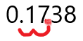
We get: 17.38% for the answer.
Convert 0.7 to a percent.
Solution
We want to move the decimal two places to the right, but there is only one digit to the right of the decimal place. The good news is that we can always add a 0 to the right of the last digit. We write:
\[0.7 = 0.70 \nonumber\]
Now move the decimal place two digits to the right to get 70%.
In regression analysis (which will be discussed MUCH later), an important number that is calculated is called R-Squared. It helps us determine how helpful one variable is in predicting another variable. The computer and calculator always display it as a decimal, but it is more meaningful as a percent. Suppose that the R-Squared value that relates the amount of studying students do to prepare for a final exam and the score on the exam is: \(r^2=0.8971\). Convert this to a percent rounded to the nearest whole number percent.
Solution
We move the decimal 0.8971 two places to the right to get 89.71%
Now round to the nearest whole number percent. Note that the digit to the left of the whole number is 7 > 5. Thus we add 1 to the whole number, 89. This gives us 90%.
Transforming a Percent to a Decimal
To convert a decimal to a percent, we multiply the decimal by 100 which is equivalent to moving the decimal two places to the right. Not surprisingly, to convert a percent to a decimal, we do exactly the opposite. We divide the number by 100 which is equivalent to moving the decimal two places to the left.
Convert the percent 89.4% to a decimal.
Solution
We move the decimal over two to the left as shown below.

We get: 0.894 for the answer.
Suppose that you want to find the value of \(x\) such that 2.5% of the entire area under a frequency line graph lies to the left of \(x\). The first step will be to convert the 2.5% to a decimal. What decimal is equivalent to 2.5%?
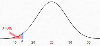
Solution
We want to move the decimal 2.5 two places to the left, but since there is only one digit to the left of the decimal, we add a zero first: 02.5. Now move the decimal two places to the left to get 0.025.
Converting a Fraction to a Decimal and a Percent
Often in probability it is natural to represent probabilities as fractions, but it is easier to make comparisons as decimals. Thus, we need to be able to convert fractions to decimals. To do so we just divide.
Find the percentage of club members attended an end-of-year event if four showed up out of seven active club members.
Solution
\[(x/N)\times100\nonumber\]
\[(\frac{4}{7} \times100) = (0.57142 \times100) = 57.14\nonumber\]
Note that we do not round up because the test number is lower than 5.
The percentage of club members who attended the end-of-year event was 57.14%.
In statistics we need to find basic probabilities and create a table for them. Suppose that you roll two six-sided dice, what percent of the time will the sum equal to a 4? Round to the nearest whole number percent.
Solution
First, notice that there are 36 total possibilities for rolling the dice, since there are 6 faces on the first die and for each value of the first die roll, there are 6 possibilities for the second die roll. Multiplying: 6 x 6 = 36. This will be the denominator. To find the numerator, we list all the possible outcome where the sum is 4:
(1,3), (2,2), and (3,1)
There are three possible outcomes with the sum equaling a 4. Thus:
\[P(\text{sum} = 4) = 3/36 \nonumber\]
Now we divide:
\[\frac{3}{36}\:=\:0.08333... \nonumber\]
Next to convert this decimal to a percent, we move the decimal two places to the right to get: 8.333...%
We are asked to round to the nearest whole number percent. The digit to the right or the whole number (8) is a 3. Since 3 < 5, we can just erase everything to the left of the 8 and leave the 8 unchanged to get 8%. Thus there is an 8% chance of getting a sum of 4 if you roll two six sided dice.
Conclusion
You won't always need to find a percentage, but keep track of this page the following resource links for when they do come back. Like all math, you lose it if you don't use it! One key to being successful is to keep track (and use!) your resources! You're usually not expected to have all of this memorized, especially at first. But you are expected to be able to find your notes and resources on how to do what you've already learned.
The following link to videos for each of these topics.
One last note: The computer or calculator shows numbers as decimals, but for presentations, percents are friendlier. It is also much easier to compare decimals than fractions, thus converting to a decimal is helpful. For example, we often want to see if a probability is greater than 5%. A computer will display the probability as a decimal such as 0.04836. To make the comparison we will first change it to a percent and then compare it to 5%.
And now we'll move back to interpreting standard deviations!