4.4: Interpreting Standard Deviations

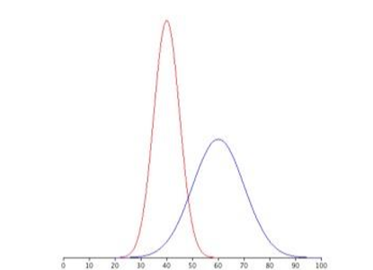
Figure \(\PageIndex{1}\) shows two symmetrical distributions. The frequency distribution on the left (red) has a mean of 40 and a standard deviation of 5; the frequency distribution on the right (blue) has a mean of 60 and a standard deviation of 10. For the tall and narrow distribution on the left, 68% of the distribution is between 45 and 55; for the shorter distribution on the right, 68% is between 50 and 70. Remember that the standard deviation shows how different each scores is, on average, from the mean. Notice that as the standard deviation gets smaller, the distribution becomes much narrower, regardless of where the center of the distribution (mean) is. The smaller standard deviation and the narrower distribution both show that the difference from the mean, on average, is smaller.

Figure \(\PageIndex{1}\): Symmetrical distributions with standard deviations of 5 and 10. (CC-BY-NC-SA Foster et al. from An Introduction to Psychological Statistics)

The next figure, Figure \(\PageIndex{2}\) was in the Introduction to Measures of Variability section. In Figure Panel (a), the mean and standard deviations are both the same. You can see where the name “bell curve” comes from: it looks a bit like a bell. In Panel (b), the mean of one of the distributions of data (red, on the right) is higher than the mean of the other distribution (blue, on the left) but the standard deviations are the same as shown by these distributions have the same “width”. The only difference between them is that they’ve been shifted to the left or to the right because the means of each distribution are different; in every other respect, they’re identical.

In contrast, if we increase the standard deviation while keeping the mean constant, the peak of the distribution stays in the same place, but the distribution gets taller, as you can see in Figure \(\PageIndex{2}\)‘s Panel (c); the means are the same (because the center of both distributions are in the same place on the x-axis), but one standard deviation is smaller (red, tall and narrow) then the other standard deviation (blue, bell shaped). The smaller standard deviation tells us that the scores, on average, are close to the mean. Notice, though, that when a distribution gets taller, the width shrinks (it gets narrower). Finally, Panel (d) shows two distributions of data in which both the means are different and the standard deviations are different (as discussed in the first Figure \(\PageIndex{1}\)).

Figure \(\PageIndex{2}\): Differences between two datasets. (CC-BY-NC-SA Foster et al. from An Introduction to Psychological Statistics)

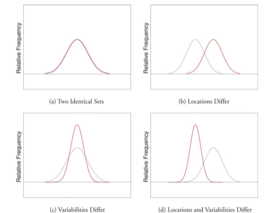
Panel (c) and Panel (d) of Figure \(\PageIndex{2}\) show that standard deviations can help us know the shape of a distribution’s frequency line graph. In other words, standard deviations can be used to predict if a frequency distribution will be skewed or have kurtosis. See the section in the chapter on graphing that discusses Skew & Kurtosis as a reminder. A small standard deviation suggests that the shape of the distribution is leptokurtic. That’s the tall and narrow (red) distribution in Panel (c) and Panel (d) of Figure \(\PageIndex{2}\). A medium standard deviation suggests that the shape of the distribution is normal or bell-shaped, sometimes called mesokurtic. That’s the bell-shaped (blue) distribution in Panel (c) and Panel (d) of Figure \(\PageIndex{2}\).

Simple enough? It gets a little more complicated when you have a large standard deviation. A large standard deviation suggestions either:

• The shape of a distribution is skewed, or
• The shape of the distribution is platykurtic (wide and flat).

A few things to note with these statements. First, just knowing that you have a large standard deviation doesn’t tell you which of these two options is true! However, the measures of central tendency from the previous chapter can be used to decide whether you think that a large standard suggests a skewed distribution of platykurtic distribution. If the mean is pretty different from the mode (the highest peak on the graph) and/or the median (the exact middle score) and your standard deviation is large, then your frequency distribution is probably skewed. Look at the skewed distribution in Figure \(\PageIndex{3}\) from the Skew and Kurtosis section of the chapter on graphs to see how these measures might interact.

Figure \(\PageIndex{3}\)- Diagram of Skew. (CC-BY-SA Rodolfo Hermans (Godot), CC BY-SA 3.0, via Wikimedia Commons)

When a distribution has a large standard deviation with a mean that’s different from the mode and/or median, you still can’t tell whether the distribution is positively or negatively skewed by just looking at the standard deviation. For example, you can’t tell whether the frequency distribution is more like the negative skew on the left or the positive skew on the right of Figure \(\PageIndex{3}\). To determine the type of skew, you’d have to look at how the three measures of central tendency relate; the large standard deviation is just a clue that the frequency distribution may be skewed (see Interpreting Measures of Central Tendency for a review).

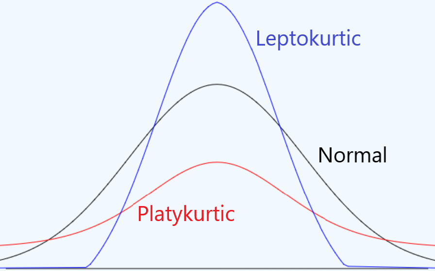
Finally, if the measures of central tendency are close together and your standard deviation is large, then your frequency distribution is probably platykurtic. You can see in Figure \(\PageIndex{4}\) (which is the same figure in the Skew and Kurtosis section in the chapter graphs) that a large standard deviation (which means that each score is, on average, far from the mean in the center) would be platykurtic and that a small standard deviation (showing that each score, on average, is close to the mean in the center) would be leptokurtic.

Figure \(\PageIndex{4}\)- Diagram of Three Kurtosis Types in Line Graphs (CC-BY Larry Green)

Small, Medium, or Large?

You’re probably still wrapping your head around how the measures of central tendency and the standard deviation can help understand the shape of a frequency distribution. I encourage you to create your own decision tree flow chart to follow the logic through all that. But while trying to piece together how the size of the standard deviation relates to the shape of a frequency chart, you might’ve wondered: how can you tell if your SD is large, medium, or small?! There’s no definitive answer to that! However, Dr. MO will provide some guidelines.

Large

First, let’s start with how to decide if a standard deviation is large because that is the more complicated decision. A general guideline (not a rigid rule) is that a standard deviation that is more than about a quarter or third of the mean is considered “large”. The next sub-section will walk you through fractions and decimals, in case this next bit gets a little to math-y for you! The general idea is that you can divide the mean by 4 (a quarter) or 3 (a third), then compare that result to the standard deviation. If the standard deviation is bigger than the mean divided by 3 or 4, then the standard deviation could be considered large. Dr. MO hasn’t seen this written anywhere, but she has decades of experience working with means and standard deviations to come up with this guideline.

If the mean is 24, then:

\[\frac{12}{4} = 6 \nonumber\]
\[\frac{12}{3} = 8 \nonumber\]

That means that the standard deviation would have to be bigger than 6 to 8 to be considered a large standard deviation.

Example \(\PageIndex{1}\)

1. If the mean is 10, would a standard deviation of 1.5 be considered large? Why or why not?
2. If the mean is 50, would a standard deviation of 18 be considered large? Why or why not?

Solution

1. Since 10 divided by 4 is 2.50 and 10 divided by 3 is 3.33, a standard deviation of 1.5 is not bigger than either of those two, so this standard deviation would not be considered large. (Stay tuned for how to determine what size it might be!)
2. Since 50 divided by 4 is 12.50 and 50 divided by 3 is 16.67 and, the standard deviation of 18 would be larger than those, so we could classify it as a large standard deviation.

Now, you can do the math on your own to see if you can decide if the standard deviation is large or not.

Exercise \(\PageIndex{1}\)

If the mean is 100, would a standard deviation of 20 be considered large? Why or why not?

Answer

Since 100 divided by 4 is 25.00 and 100 divided by 3 is 33.33, a standard deviation of 20 is not bigger than either of those two, so the standard deviation of 8 would not be considered large. (Stay tuned for how to determine what size it might be!)

Sometimes students try to look at just the standard deviation to use it to predict the shape of a distribution, but this is missing necessary context. The standard deviation on its own isn’t all that useful; you need to know the central tendencies (especially the average scores), to decide. But as the examples above show, sometimes 18 is a large standard deviation and sometimes 20 is not a large standard deviation! It all depends on the data you are working with.

Before we move on, here’s a reminder that finding a large standard deviation is just a piece of the puzzle. To try to predict the shape of the distribution, you’d need to compare the large standard deviation with the measures of central tendency to determine if that large standard deviation suggests a skewed distribution or a kurtosis that is wide and flat (platykurtic).

Small

Okay, let’s figure out how to estimate if the standard deviation could be considered small. You’ll see next why we’ll talk about medium-sized standard deviations last! Dr. MO felt pretty confident about sharing the quarter-to-a-third general guideline to identify large standard deviations, but she’s less confident in generating a guideline for identifying a small standard deviation. The best that she can come up with is if the standard deviation is less than 10% of the mean, then it’s probably a small standard deviation.

If the mean is 24, then you’d multiply that by .10 (which is the decimal for 10%).

\[24 \times 0.10= 2.40 \nonumber\]

That means that the standard deviation would have to be smaller than 2.40 to be considered a small standard deviation. If you’re a little lost on how to get from a percentage to a decimal (or vice versa), you are highly encouraged to review the next section.

Example \(\PageIndex{2}\)

1. If the mean is 10, would a standard deviation of 1.5 be considered small? Why or why not?
2. If the mean is 50, would a standard deviation of 18 be considered small? Why or why not?

Solution

1. A standard deviation of 1.5 is not smaller 1.00, which is 10% of 10 (10 times 0.10 is 1.00), so this standard deviation would not be considered small. (Stay tuned for how to determine what size it might be!)
2. Since 50 times 0.10 is 5, then a standard of 18 would also not be smaller, so this standard deviation would also not be considered small.

Try it yourself!

Exercise \(\PageIndex{2}\)

If the mean is 100, would a standard deviation of 20 be considered small? Why or why not?

Answer

Since 10% of 100 is 10 (100 times 0.10 is 10), a standard deviation of 20 is also not smaller, so the standard deviation of 20 would not be considered small.

Exercise \(\PageIndex{3}\)

What kurtosis would we predict with a small standard deviation?.

Answer

Small standard deviations suggest that each score, on average, is similar to the mean. This would be a leptokurtic frequency distribution, which is tall and narrow.

Medium

How do you decide if a standard deviation is medium-sized? Basically, if your standard deviation is not large and is not small, then it’s medium!

Exercise \(\PageIndex{4}\)

What kurtosis would we predict with a medium standard deviation?

Answer

Medium standard deviations suggest a mesokurtic frequency distribution, which is shaped like a bell.

Conclusion

Understanding the relationships amongst the measures of central tendencies and the standard deviation (as a measure of variability), is a major way to show that your math literacy. After the sub-section on fractions, you can practice all of this, plus refresh on using just the three measures of central tendency to predict the shape of a distribution.

Contributors

• Foster et al. (University of Missouri-St. Louis, Rice University, & University of Houston, Downtown Campus)

• Dr. MO (Taft College)