3.6: Interpreting All Three

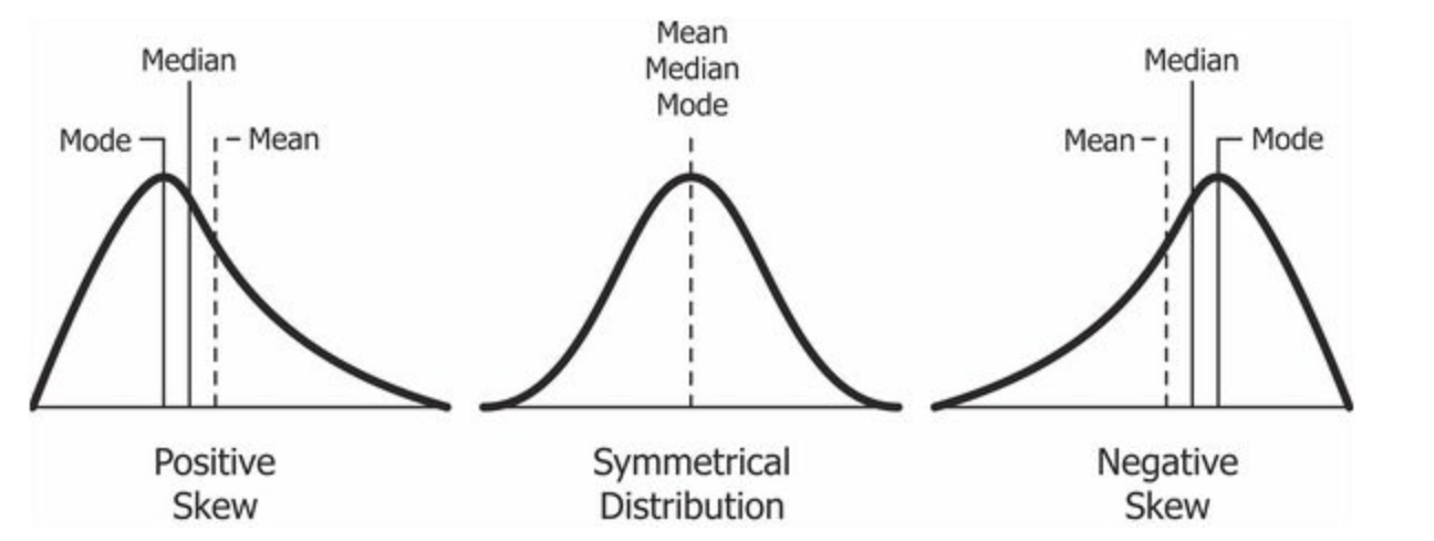
In a symmetrical, unimodal distribution, the mode, median, and mean are all the same number.

Note

What does symmetrical mean?

What does unimodal mean?

This means that the more symmetrical a distribution is, the closer the median, mode, and mean will be.

By knowing how similar the median, mode, and mean are, you can guesstimate at the symmetricalness of the distribution.

Example \(\PageIndex{1}\)

What’s skew? Positive skew? Negative skew?

Solution

Find these terms in the glossary, or the parts of this chapter when skew was discussed.

Without having all of the data or seeing the distribution, we can make predictions about what the distribution might look like because:

• The mean is pulled in the direction of the extreme scores (or tail of the skew),
• The mode is the highest point in the skew,
• The median is between the mean and mode.

In particular, we can predict that:

• If the mean is a lot bigger than the median, that the distribution will have a positive skew.
  • Mean > Median = positive skew
• If the mean is a lot smaller than the median, that the distribution will have a negative skew.
  • Mean < Median = negative skew

Figure \(\PageIndex{1}\): Mean, Median, Mode, and Skew (Copyright CC-BY-SA Diva Jain/Diva Dugar, Source)

Practice

We'll use the data in Table \(\PageIndex{1}\) to practice calculating and interpreting the measures of central tendency. The first column (labeled "Student") just identifies the student by an identification number. These identification numbers may not be meaningful data or they could be student names, but this column also indicates that all information in that row (left to right) is information about that same student. We will first practice calculating and interpreting the measures of central tendency together on the Final Grade Percentage column of this is real data from a section of Dr. MO's behavioral statistics class, and then you can practice calculating and interpreting the measures of central tendency yourself for the Number of Absences variable. But before we begin, why can't we interpret the three measures of central tendency for the column showing each students major?

Example \(\PageIndex{2}\)

Calculate the measures of central tendency for student's major in Table \(\PageIndex{1}\).

Hint: Some of this question is a trick question?

1. Mean
2. Median
3. Mode

Solution

1. Mean: While a spreadsheet will show the sum of the student's major as zero, you should recognize that you can't add together qualitative data. Thus, you could do the math to calculate a mean, but it wouldn't make sense.

\[\bar{X} = {\dfrac{\sum X}{N}} = {\dfrac{0}{9}} = 0 \nonumber \]

2. Median: Similarly, to find the middle number you must have numbers in numerical order. Since Major is a qualitative variable, we can put it in alphabetical order but no numerical order.
3. Mode: We do have a mode! The most frequent answer is Education, so the mode of these student's major is Education. I did ask Excel to find the mode, though, and it said that it was "not available." Again, it's important to understand the kind of variable you have and the limitations of the software you are using!

Reviewing Example \(\PageIndex{2}\), you should notice that we really only can calculate one measure of central tendency for the variable of student major in Table \(\PageIndex{1}\) since student major is a qualitative variable. So, why can't we interpret the three measures of central tendency for the column showing each students major? Because we can only find one measure of central tendency (mode) for qualitative variables.

Table \(\PageIndex{1}\): Prior Class Data

Student	Major	Final Grade Percentage	Number of Absences
1	Business	83.6	5
2	Business	73.4	4
3	Criminal Justice	82.9	8
4	Criminal Justice	72.4	9
5	Education	86.0	2
6	Education	83.9	7
7	Education	83.0	4
8	Psychology	36.0	25
9	Psychology	36.0	17
\(\Sigma =\)	\(\Sigma = 0\)	\(\Sigma = 637.20\)	\(\Sigma = 81.00\)

Practice: Final Grade Percentage

Okay, let's move on to a variable that we can calculate all three measures of central tendency, and then see what they are trying to tell us.

Example \(\PageIndex{2}\)

To interpret the scenario and measures of central tendency for Final Grade Percentage provided in Table \(\PageIndex{1}\), answer the following questions.

1. Who is the sample? Include as much information as you have (such as number in the sample, course, and professor).
2. Who could be the population? In other words, what’s the biggest group that this sample could represent?
3. What is the mean, median, and mode for Final Grade Percentage?
   1. Hint: For the median, create a frequency table.
4. If we couldn’t see all of the data in Table \(\PageIndex{1}\) but knowing the measures of central tendency (mean, median, & mode), do you think that the frequency distribution will be positively skewed, negatively skewed, or not skewed? In other words what would we guess that the frequency line graph for the Final Grade Percentage will look like based on these measures of central tendency?

Solution

1. The sample is nine students from a section of Dr. MO's behavioral statistics course.
2. The population could be all students in behavioral statistics courses. The population could also be all students from the same college, or all students in Dr. MO's behavioral statistics courses through time. There's not one right answer for who could be the population, it just has to make sense.
3. For Final Grade Percentage:
   1. Mean: \[\bar{X} = {\dfrac{\sum X}{N}} = {\dfrac{637.20}{9}} = 70.80 \nonumber \]
   2. Median: The exact middle score is 82.90
      1. You have to put the scores in numerical order to find the one that is in the middle.
   3. Mode: The most frequent score is 36.00.
4. Because the mode is so small, I would predict that the shape of the distribution is positively skewed. The mean responds to extreme scores, so usually the mean is closer to the tail of the distribution than the median. When the mean is smaller than the median, you would predict a a negative skew (see Figure \(\PageIndex{1}\)). With these competing predictions for skew, there's no way to predict the skew or shape of the distribution. This often happens with small distributions.

Despite the measures of central tendency not being useful to predict the shape of the graph (probably due to our small sample size), you can see in Figure \(\PageIndex{2}\) that the distribution is positively skewed. And before you get worried that the mode is such a low final grade, notice that the rest of the grades are passing. There were two students who stopped attending class during the first month, and those were the only two students who did not pass the course! When you have a small sample, a couple extreme scores can really change the whole interpretation.

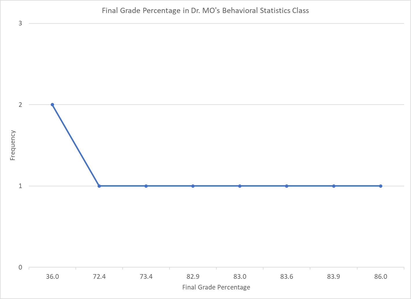
Figure \(\PageIndex{2}\): Line Graph of Frequency of Final Grade Percentages. (Copyright CC-SA, chart by Dr. MO via class data)

Practice: Absences

It's your turn now!

Exercise \(\PageIndex{1}\)

To interpret the scenario and measures of central tendency for Absences provided in Table \(\PageIndex{1}\), answer the following questions.

1. Who is the sample? Include as much information as you have (such as number in the sample, course, and professor).
   1. Hint: This is the same as above since it's the same people in the sample.
2. Who could be the population? In other words, what’s the biggest group that this sample could represent?
   1. 1. Hint: This could the same as above since it's the same people in the sample
3. What is the mean, median, and mode for Final Grade Percentage?
   1. Hint: For the median, create a frequency table.
4. If we couldn’t see all of the data in Table \(\PageIndex{1}\) but knowing the measures of central tendency (mean, median, & mode), do you think that the frequency distribution will be positively skewed, negatively skewed, or not skewed? In other words what would we guess that the frequency line graph for the Final Grade Percentage will look like based on these measures of central tendency?

Answer

1. The sample is nine students from a section of Dr. MO's behavioral statistics course.
2. The population could be all students in behavioral statistics courses. The population could also be all students from the same college, or all students in Dr. MO's behavioral statistics courses through time. There's not one right answer for who could be the population, it just has to make sense.
3. For Absences:
   1. Mean: \[\bar{X} = {\dfrac{\sum X}{N}} = {\dfrac{81}{9}} = 9 \nonumber \]
   2. Median: The exact middle score is 7.00
      1. You have to put the scores in numerical order to find the one that is in the middle.
   3. Mode: The most frequent score is 4.
4. Because the mode is smaller than the median and mean, and the mean seems be pulled higher by extreme scores, I would predict that the shape of the distribution is positively skewed.

Look at the distribution in Figure \(\PageIndex{3}\) to see if your prediction was correct:

Figure \(\PageIndex{3}\): Line Graph of Frequency of Absences. (Copyright CC-SA, chart by Dr. MO via class data)

While we are not analyzing whether absences are related to final grades, Table \(\PageIndex{1}\) seems to suggest that the two students who missed a lot of classes (making our average number of absences really high!) are also the two students who did not pass the course. In sum, attend your classes!

Conclusion

Although you've learned about the measures of central tendency before, this section shows you how we can use these three numbers together to understand what a whole distribution of data might tell us.

In the next chapter, we'll look at measures of variability that, combined with the measures of central tendency, will tell us a LOT about a distribution of data.