
10.3: Increasing Satisfaction at Work
- Page ID
- 14510

Workers at a local company have been complaining that working conditions have gotten very poor, hours are too long, and they don’t feel supported by the management. The company hires a consultant to come in and help fix the situation before it gets so bad that the employees start to quit. The consultant first assesses 40 of the employee’s level of job satisfaction as part of focus groups used to identify specific changes that might help. The company institutes some of these changes, and six months later the consultant returns to measure job satisfaction again. Knowing that some interventions miss the mark and can actually make things worse, the consultant tests for a difference in either direction (i.e. and increase or a decreased in average job satisfaction) at the \(α\) = 0.05 level of significance.
Step 1: State the Hypotheses:
First, we state our null and alternative hypotheses:
\(H_0\): There is no increase in average job satisfaction after the changes
\(H_0: μ_D \leq 0\)
\(H_A\): There is an increase in average job satisfaction after the changes
\(H_A: μ_D > 0\)
In this case, we are hoping that the changes we made will improve employee satisfaction, and, because we based the changes on employee recommendations, we have good reason to believe that they will. Thus, we will use a one-directional alternative hypothesis.
Step 2: Find the Critical Values:
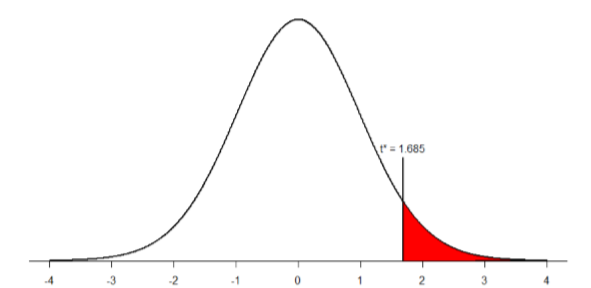
Our critical values will once again be based on our level of significance, which we know is \(α\) = 0.05, the directionality of our test, which is one-tailed to the right, and our degrees of freedom. For our dependent-samples \(t\)-test, the degrees of freedom are still given as \(df = n – 1\). For this problem, we have 40 people, so our degrees of freedom are 39. Going to our t-table, we find that the critical value is \(t*\) = 1.685 as shown in Figure \(\PageIndex{1}\).
Step 3: Calculate the Test Statistic:
Now that the criteria are set, it is time to calculate the test statistic. The data obtained by the consultant found that the difference scores from time 1 to time 2 had a mean of \(M_{\mathrm{D}}\) = 2.96 and a standard deviation of \(s_D\) = 2.85. Using this information, plus the size of the sample (\(N\) = 40), we first calculate the standard error:
\[s_{M_{D}}=s_{D / \sqrt{n}}=2.85 / \sqrt{40}=2.85 / 6.32=0.46 \nonumber \]
Now, we can put that value, along with our sample mean and null hypothesis value, into the formula for \(t\) and calculate the test statistic:
\[t=\dfrac{M_{D}-\mu_{D}}{s_{M_{D}}}=\dfrac{2.96-0}{0.46}=6.43 \nonumber \]
Notice that, because the \(μ_D\) of a paired samples \(t\)-test is 0, we can simply divide our obtained sample mean by the standard error.
Step 4: Make the Decision:
We have obtained a test statistic of \(t\) = 6.43 that we can compare to our previously established critical value of \(t*\) = 1.685. 6.43 is larger than 1.685, so \(t > t*\) and we reject the null hypothesis:
Reject \(H_0\). Based on the sample data from 40 workers, we can say that the intervention statistically significantly improved job satisfaction (\(M_{\mathrm{D}}\)= 2.96) among the workers, \(t(39) = 6.43\), \(p < 0.05\).
Because this result was statistically significant, we will want to calculate Cohen’s \(d\) as an effect size using the same format as we did for the last \(t\)-test:
\[t=\dfrac{M_{D}-\mu_{D}}{s_{D}}=\dfrac{2.96}{2.85}=1.04 \nonumber \]
This is a large effect size. Notice again that we can omit the \( μ_D \) here because it is equal to 0.
Hopefully the above example made it clear that running a paired samples \(t\)-test to look for differences before and after some treatment works exactly the same way as a regular 1-sample \(t\)-test does, which was just a small change in how \(z\)-tests were performed in chapter 7. At this point, this process should feel familiar, and we will continue to make small adjustments to this familiar process as we encounter new types of data to test new types of research questions.
Contributors and Attributions
Foster et al. (University of Missouri-St. Louis, Rice University, & University of Houston, Downtown Campus)