
13.3: Three Characteristics
- Page ID
- 14537

When we talk about correlations, there are three traits that we need to know in order to truly understand the relation (or lack of relation) between \(X\) and \(Y\): form, direction, and magnitude. We will discuss each of them in turn.
Form
The first characteristic of relations between variables is their form. The form of a relation is the shape it takes in a scatterplot, and a scatterplot is the only way it is possible to assess the form of a relation. There are three forms we look for: linear, curvilinear, or no relation. A linear relation is what we saw in Figures 12.2.1, 12.2.2, and 12.2.3. If we drew a line through the middle points in the any of the scatterplots, we would be best suited with a straight line. The term “linear” comes from the word “line”. A linear relation is what we will always assume when we calculate correlations. All of the correlations presented here are only valid for linear relations. Thus, it is important to plot our data to make sure we meet this assumption.
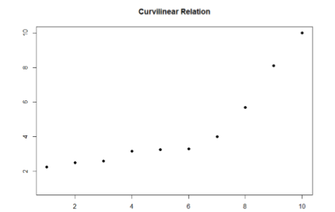
The relation between two variables can also be curvilinear. As the name suggests, a curvilinear relation is one in which a line through the middle of the points in a scatterplot will be curved rather than straight. Two examples are presented in Figures \(\PageIndex{1}\) and \(\PageIndex{2}\).
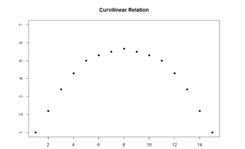
Curvilinear relations can take many shapes, and the two examples above are only a small sample of the possibilities. What they have in common is that they both have a very clear pattern but that pattern is not a straight line. If we try to draw a straight line through them, we would get a result similar to what is shown in Figure \(\PageIndex{3}\).
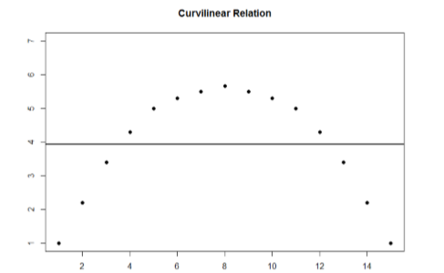
Although that line is the closest it can be to all points at the same time, it clearly does a very poor job of representing the relation we see. Additionally, the line itself is flat, suggesting there is no relation between the two variables even though the data show that there is one. This is important to keep in mind, because the math behind our calculations of correlation coefficients will only ever produce a straight line – we cannot create a curved line with the techniques discussed here.
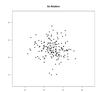
Finally, sometimes when we create a scatterplot, we end up with no interpretable relation at all. An example of this is shown below in Figure \(\PageIndex{4}\). The points in this plot show no consistency in relation, and a line through the middle would once again be a straight, flat line.
Sometimes when we look at scatterplots, it is tempting to get biased by a few points that fall far away from the rest of the points and seem to imply that there may be some sort of relation. These points are called outliers, and we will discuss them in more detail later in the chapter. These can be common, so it is important to formally test for a relation between our variables, not just rely on visualization. This is the point of hypothesis testing with correlations, and we will go in depth on it soon. First, however, we need to describe the other two characteristics of relations: direction and magnitude.
Direction
The direction of the relation between two variables tells us whether the variables change in the same way at the same time or in opposite ways at the same time. We saw this concept earlier when first discussing scatterplots, and we used the terms positive and negative. A positive relation is one in which \(X\) and \(Y\) change in the same direction: as \(X\) goes up, \(Y\) goes up, and as \(X\) goes down, \(Y\) also goes down. A negative relation is just the opposite: \(X\) and \(Y\) change together in opposite directions: as \(X\) goes up, \(Y\) goes down, and vice versa.
As we will see soon, when we calculate a correlation coefficient, we are quantifying the relation demonstrated in a scatterplot. That is, we are putting a number to it. That number will be either positive, negative, or zero, and we interpret the sign of the number as our direction. If the number is positive, it is a positive relation, and if it is negative, it is a negative relation. If it is zero, then there is no relation. The direction of the relation corresponds directly to the slope of the hypothetical line we draw through scatterplots when assessing the form of the relation. If the line has a positive slope that moves from bottom left to top right, it is positive, and vice versa for negative. If the line it flat, that means it has no slope, and there is no relation, which will in turn yield a zero for our correlation coefficient.
Magnitude
The number we calculate for our correlation coefficient, which we will describe in detail below, corresponds to the magnitude of the relation between the two variables. The magnitude is how strong or how consistent the relation between the variables is. Higher numbers mean greater magnitude, which means a stronger relation.
Our correlation coefficients will take on any value between -1.00 and 1.00, with 0.00 in the middle, which again represents no relation. A correlation of -1.00 is a perfect negative relation; as \(X\) goes up by some amount, \(Y\) goes down by the same amount, consistently. Likewise, a correlation of 1.00 indicates a perfect positive relation; as \(X\) goes up by some amount, \(Y\) also goes up by the same amount. Finally, a correlation of 0.00, which indicates no relation, means that as \(X\) goes up by some amount, \(Y\) may or may not change by any amount, and it does so inconsistently.
The vast majority of correlations do not reach -1.00 or positive 1.00. Instead, they fall in between, and we use rough cut offs for how strong the relation is based on this number. Importantly, the sign of the number (the direction of the relation) has no bearing on how strong the relation is. The only thing that matters is the magnitude, or the absolute value of the correlation coefficient. A correlation of -1 is just as strong as a correlation of 1. We generally use values of 0.10, 0.30, and 0.50 as indicating weak, moderate, and strong relations, respectively.
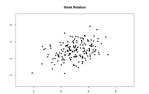
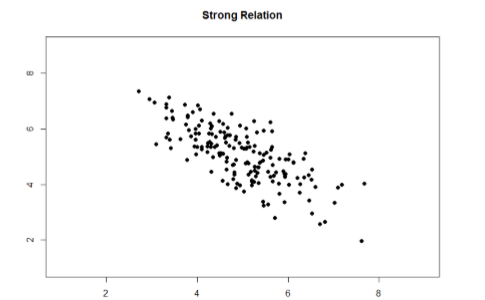
The strength of a relation, just like the form and direction, can also be inferred from a scatterplot, though this is much more difficult to do. Some examples of weak and strong relations are shown in Figures \(\PageIndex{5}\) and \(\PageIndex{6}\), respectively. Weak correlations still have an interpretable form and direction, but it is much harder to see. Strong correlations have a very clear pattern, and the points tend to form a line. The examples show two different directions, but remember that the direction does not matter for the strength, only the consistency of the relation and the size of the number, which we will see next.
Contributors and Attributions
Foster et al. (University of Missouri-St. Louis, Rice University, & University of Houston, Downtown Campus)