5.6: Poisson Distribution

Last updated
Save as PDF

Page ID: 16253

$ \newcommand{\vecs}[1]{\overset { \scriptstyle \rightharpoonup} {\mathbf{#1}} } $ $ \newcommand{\vecd}[1]{\overset{-\!-\!\rightharpoonup}{\vphantom{a}\smash {#1}}} $$\newcommand{\id}{\mathrm{id}}$ $ \newcommand{\Span}{\mathrm{span}}$ $ \newcommand{\kernel}{\mathrm{null}\,}$ $ \newcommand{\range}{\mathrm{range}\,}$ $ \newcommand{\RealPart}{\mathrm{Re}}$ $ \newcommand{\ImaginaryPart}{\mathrm{Im}}$ $ \newcommand{\Argument}{\mathrm{Arg}}$ $ \newcommand{\norm}[1]{\| #1 \|}$ $ \newcommand{\inner}[2]{\langle #1, #2 \rangle}$ $ \newcommand{\Span}{\mathrm{span}}$ $\newcommand{\id}{\mathrm{id}}$ $ \newcommand{\Span}{\mathrm{span}}$ $ \newcommand{\kernel}{\mathrm{null}\,}$ $ \newcommand{\range}{\mathrm{range}\,}$ $ \newcommand{\RealPart}{\mathrm{Re}}$ $ \newcommand{\ImaginaryPart}{\mathrm{Im}}$ $ \newcommand{\Argument}{\mathrm{Arg}}$ $ \newcommand{\norm}[1]{\| #1 \|}$ $ \newcommand{\inner}[2]{\langle #1, #2 \rangle}$ $ \newcommand{\Span}{\mathrm{span}}$$\newcommand{\AA}{\unicode[.8,0]{x212B}}$

There are two main characteristics of a Poisson experiment.

The Poisson probability distribution gives the probability of a number of events occurring in a fixed interval of time or space if these events happen with a known average rate and independently of the time since the last event. For example, a book editor might be interested in the number of words spelled incorrectly in a particular book. It might be that, on the average, there are five words spelled incorrectly in 100 pages. The interval is the 100 pages.
The Poisson distribution may be used to approximate the binomial if the probability of success is “small” (such as 0.01) and the number of trials is “large” (such as 1,000). You will verify the relationship in the homework exercises. n is the number of trials, and p is the probability of a “success.”

The random variable $X=$ the number of occurrences in the interval of interest.

Example 1:

The average number of loaves of bread put on a shelf in a bakery in a half-hour period is 12. Of interest is the number of loaves of bread put on the shelf in five minutes. The time interval of interest is five minutes. What is the probability that the number of loaves, selected randomly, put on the shelf in five minutes is three?

Solution:

Let $X=$ the number of loaves of bread put on the shelf in five minutes. If the average number of loaves put on the shelf in 30 minutes (half-hour) is 12, then the average number of loaves put on the shelf in five minutes is $\left(\frac{5}{30}\right)\left(12\right)=2$ loaves of bread.

The probability question asks you to find $P(x=3)$ .

Notation for the Poisson: $P=$ Poisson Probability Distribution Function

$X{\sim}P(\mu)$

Read this as “X is a random variable with a Poisson distribution.” The parameter is μ (or λ); μ (or λ) $=$ the mean for the interval of interest.

Example 2:

Leah’s answering machine receives about six telephone calls between 8 a.m. and 10 a.m. What is the probability that Leah receives more than one call in the next 15 minutes?

Solution:

Let $X=$ the number of calls Leah receives in 15 minutes. (The interval of interest is 15 minutes or 14 hour.)

$x=0,1,2,3,...$

If Leah receives, on the average, six telephone calls in two hours, and there are eight 15 minute intervals in two hours, then Leah receives $(18)(6)=0.75$ calls in 15 minutes, on average. So, $\mu=0.75$ for this problem.

$X ~ P(0.75)$

Find P(x > 1). P(x > 1) = 0.1734 (calculator or computer)

Press 1 – and then press 2^nd DISTR.
Arrow down to poissoncdf. Press ENTER.
Enter (.75,1).
The result is P(x > 1) = 0.1734.

NOTE

The TI calculators use λ (lambda) for the mean.

The probability that Leah receives more than one telephone call in the next 15 minutes is about 0.1734:

P(x > 1) = 1 − poissoncdf(0.75, 1).

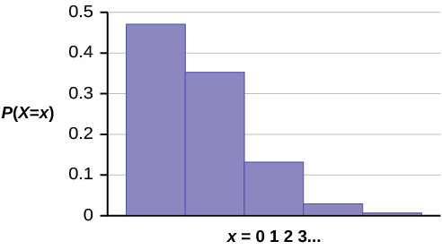
The graph of X ~ P(0.75) is:

This graphs shows a poisson probability distribution. It has 5 bars that decrease in height from left to right. The x-axis shows values in increments of 1 starting with 0, representing the number of calls Leah receives within 15 minutes. The y-axis ranges from 0 to 0.5 in increments of 0.1.

The y-axis contains the probability of x where X = the number of calls in 15 minutes.

Example 3:

According to Baydin, an email management company, an email user gets, on average, 147 emails per day. Let X = the number of emails an email user receives per day. The discrete random variable X takes on the values x = 0, 1, 2 …. The random variable Xhas a Poisson distribution: X ~ P(147). The mean is 147 emails.

What is the probability that an email user receives exactly 160 emails per day?
What is the probability that an email user receives at most 160 emails per day?
What is the standard deviation?

Solution

P(x = 160) = poissonpdf(147, 160) ≈ 0.0180
P(x ≤ 160) = poissoncdf(147, 160) ≈ 0.8666
Standard Deviation = $\sigma=\sqrt{\mu}=\sqrt{144}$ ≈12.1244

Review

A Poisson probability distribution of a discrete random variable gives the probability of a number of events occurring in a fixed interval of time or space, if these events happen at a known average rate and independently of the time since the last event. The Poisson distribution may be used to approximate the binomial, if the probability of success is “small” (less than or equal to 0.05) and the number of trials is “large” (greater than or equal to 20).

Formula Review

X ~ P(μ) means that X has a Poisson probability distribution where X = the number of occurrences in the interval of interest.

X takes on the values x = 0, 1, 2, 3, …

The mean μ is typically given.

The variance is σ² = μ, and the standard deviation is σ = $\sqrt{\mu}$ .

When P(μ) is used to approximate a binomial distribution, μ = np where n represents the number of independent trials and p represents the probability of success in a single trial.

Thumbnail for the embedded element "The Poisson Distribution"

A YouTube element has been excluded from this version of the text. You can view it online here: http://pb.libretexts.org/esm/?p=84

The POisson Distribution. Provided by: OpenStax. Located at: http://cnx.org/contents/30189442-6998-4686-ac05-ed152b91b9de@17.44.. License: CC BY: Attribution. License Terms: Download for free at http://cnx.org/contents/30189442-699...2b91b9de@17.44.
Introductory Statistics . Authored by: Barbara Illowski, Susan Dean. Provided by: Open Stax. Located at: http://cnx.org/contents/30189442-6998-4686-ac05-ed152b91b9de@17.44. License: CC BY: Attribution. License Terms: Download for free at http://cnx.org/contents/30189442-699...2b91b9de@17.44

Example 1:

Solution:

Notation for the Poisson: Poisson Probability Distribution Function

Example 2:

Solution:

Example 3:

Solution

Review

Formula Review

Notation for the Poisson: $P=$ Poisson Probability Distribution Function