
2.6: Skewness and the Mean, Median, and Mode
- Page ID
- 16238
Consider the following data set.
4; 5; 6; 6; 6; 7; 7; 7; 7; 7; 7; 8; 8; 8; 9; 10
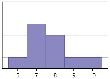
This data set can be represented by following histogram. Each interval has width one, and each value is located in the middle of an interval.
Figure 1.

The histogram displays a symmetrical distribution of data. A distribution is symmetrical if a vertical line can be drawn at some point in the histogram such that the shape to the left and the right of the vertical line are mirror images of each other. The mean, the median, and the mode are each seven for these data. In a perfectly symmetrical distribution, the mean and the median are the same. This example has one mode (unimodal), and the mode is the same as the mean and median. In a symmetrical distribution that has two modes (bimodal), the two modes would be different from the mean and median.
Consider the following data set: 4 5 6 6 6 7 7 7 7 8.
The histogram is not symmetrical.
The right-hand side seems “chopped off” compared to the left side. A distribution of this type is called skewed to the left because it is pulled out to the left.
Figure 2.

The mean is 6.3, the median is 6.5, and the mode is seven. Notice that the mean is less than the median, and they are both less than the mode. The mean and the median both reflect the skewing, but the mean reflects it more so.
Consider the following data set: 6 7 7 7 7 8 8 8 9 10.
The histogram is also not symmetrical. It is skewed to the right.
Figure 3.
The mean is 7.7, the median is 7.5, and the mode is 7.
Of the three statistics, the mean is the largest, while the mode is the smallest. Again, the mean reflects the skewing the most.
To summarize,
- if the distribution of data is skewed to the left, the mean is less than the median, which is often less than the mode.
(median < median < mode) - If the distribution of data is skewed to the right, the mode is often less than the median, which is less than the mean.
(mean > median > mode) - If the distribution of data is symmetric, the mode = the median = the mean.
Skewness and symmetry become important when we discuss probability distributions in later chapters.
Here is a video that summarizes how the mean, median and mode can help us describe the skewness of a dataset. Don’t worry about the terms leptokurtic and platykurtic for this course.

A YouTube element has been excluded from this version of the text. You can view it online here: http://pb.libretexts.org/esm/?p=52
Statistics are used to compare and sometimes identify authors. The following lists shows a simple random sample that compares the letter counts for three authors.
Terry: 7; 9; 3; 3; 3; 4; 1; 3; 2; 2
Davi: 3; 3; 3; 4; 1; 4; 3; 2; 3; 1
Mari: 2; 3; 4; 4; 4; 6; 6; 6; 8; 3
- Make a dot plot for the three authors and compare the shapes.
[reveal-answer q=”811563″]Show Answer[/reveal-answer]
[hidden-answer a=”811563″]
Terry’s distribution is right-skewed.

Davi’s distribution is slightly left-skewed.
Mari’s distribution is symmetrical.[/hidden-answer] - Calculate the mean for each.
[reveal-answer q=”379980″]Show Answer[/reveal-answer]
[hidden-answer a=”379980″]Terry’s mean is 3.7, Davi’s mean is 2.7, Mari’s mean is 4.6.[/hidden-answer] - Calculate the median for each.
[reveal-answer q=”936678″]Show Answer[/reveal-answer]
[hidden-answer a=”936678″]Terry’s median is three, Davi’s median is three. Mari’s median is four.[/hidden-answer] - Describe any pattern you notice between the shape and the measures of center.
[reveal-answer q=”75768″]Show Answer[/reveal-answer]
[hidden-answer a=”75768″]It appears that the median is always closest to the high point (the mode), while the mean tends to be farther out on the tail. In a symmetrical distribution, the mean and the median are both centrally located close to the high point of the distribution.[/hidden-answer]
Try It
Discuss the mean, median, and mode for each of the following problems. Is there a pattern between the shape and measure of the center?
a.
b.
| The Ages Former U.S Presidents Died | |
|---|---|
| 4 | 6 9 |
| 5 | 3 6 7 7 7 8 |
| 6 | 0 0 3 3 4 4 5 6 7 7 7 8 |
| 7 | 0 1 1 2 3 4 7 8 8 9 |
| 8 | 0 1 3 5 8 |
| 9 | 0 0 3 3 |
| Key: 8|0 means 80. | |
c.
[reveal-answer q=”210035″]Show Answer[/reveal-answer]
[hidden-answer a=”210035″]
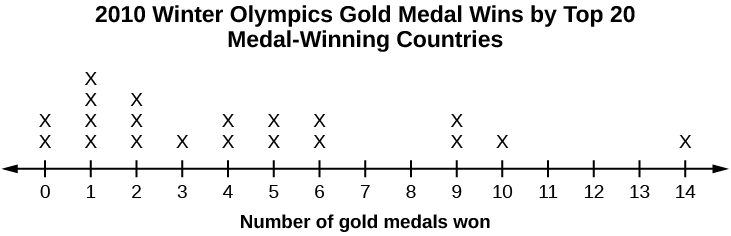
- mean = 4.25, median = 3.5, mode = 1; The mean > median > mode which indicates skewness to the right. (data are 0, 1, 2, 3, 4, 5, 6, 9, 10, 14 and respective frequencies are 2, 4, 3, 1, 2, 2, 2, 2, 1, 1)
- mean = 70.1 , median = 68, mode = 57, 67 bimodal; the mean and median are close but there is a little skewness to the right which is influenced by the data being bimodal. (data are 46, 49, 53, 56, 57, 57, 57, 58, 60, 60, 63, 63, 64, 64, 65, 66, 67, 67, 67, 68, 70, 71, 71, 72, 73, 74, 77, 78, 78, 79, 80, 81, 83, 85, 88, 90, 90 93, 93).
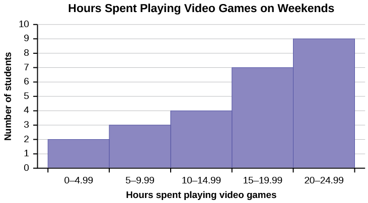
- These are estimates: mean =16.095, median = 17.495, mode = 22.495 (there may be no mode); The mean < median < mode which indicates skewness to the left. (data are the midponts of the intervals: 2.495, 7.495, 12.495, 17.495, 22.495 and respective frequencies are 2, 3, 4, 7, 9).
[/hidden-answer]
Concept Review
Looking at the distribution of data can reveal a lot about the relationship between the mean, the median, and the mode. There are three types of distributions. A right (or positive) skewed distribution has a shape like Figure 2. A left (or negative) skewed distribution has a shape like Figure 3 . A symmetrical distribution looks like Figure 1.
- Introductory Statistics. Provided by: OpenStax. Located at: http://cnx.org/contents/30189442-6998-4686-ac05-ed152b91b9de@17.44.. License: CC BY: Attribution. License Terms: Download for free at http://cnx.org/contents/30189442-699...2b91b9de@17.44
- Introductory Statistics . Authored by: Barbara Illowski, Susan Dean. Provided by: Open Stax. Located at: http://cnx.org/contents/30189442-6998-4686-ac05-ed152b91b9de@17.44. License: CC BY: Attribution. License Terms: Download for free at http://cnx.org/contents/30189442-699...2b91b9de@17.44
- Elementary Business Statistics | Skewness and the Mean, Median, and Mode. Authored by: Janux. Provided by: Janux. Located at: https://youtu.be/s6N_l3Bu-Mc. License: All Rights Reserved. License Terms: Standard YouTube License