Ch 10.1 and 10.4 Hypothesis Test for 2 Population Means

Ch 10.1 and 10.4 Hypothesis Test for 2 population means

Independent and Dependent samples

Independent samples: - sample values from one population are not related to or naturally paired or matched with the sample values from the other. Sample size can be same or different.

Summary statistics or data can be given.

 

Dependent samples: - sample values are some how matched, where the matching is based on some inherent relationship. (This can be measurement from the same subject before/after, or each pair consists of matched pairs such as husband/wife, twin of siblings.) Note: “match paired” does not mean cause/effect.

Sample size must be the same. Paired sample data will be given.

 

Note: Experiment result from dependent samples are more favorable than result from independent sample.

Ex1. sample 1: heights of 14 men.

        sample 2:  heights of 16 women.

        The above samples are independent.

 

Ex2: sample 1: Heights of husband of a couple.

         sample 2: Height of the wife of each couple.

         Since each paired value are from the same couple. The samples are dependent.

 

 

Use independent samples to compare population means

To compare population mean(μ1 and μ2) from two populations, sample means ( \( \bar{x_1} and \bar{x_2} \)  ) are collected. If  \( \bar{x_1} \) and \( \bar{x_1} \) are normally distributed, then the difference \( \bar{x_1} - \bar{x_2} \) will be also be normally distributed.

The standard deviation of \( \bar{x_1} - \bar{x_2} \)  will have a value that is square root of the sum of variances.

The most common case is both σ1 and σ2 are unknown and unequal.

Hence variances are not pooled, and sample variances are used to standardize the distribution of

  \( \bar{x_1} - \bar{x_2} \) with   \(  t =\frac{(\bar{x_1}-\bar{x_2})-(\mu _1 - \mu _2)}{ \sqrt{ \frac{(s_1)^2}{n_1}+\frac{(s_2)^2}{n_2} } } \)

   

Note: by default, when σ1 and σ2 are not given, we assume σ1 and σ2 are unknown and unequal, resulting in not pooling the variances.

 

Use paired difference (d) to compare population means.

When samples are dependent, we define a new variable d  = x1 – x2 for each paired data.

The distribution of  \( \bar{d}  \) will be normal if X1 and X2 are normal or sample size n1 = n2 = n > 30. The sample mean of d is \( \bar{d}  \) with standard deviation \( s_d \).

The distribution of \( \bar{d}  \) will have a standard deviation \(\frac{ s_d}{\sqrt{n}} \) .  Hence t distribution is used to describe the standard error  with \( t = \frac{ \bar{d} - \mu _d}{s_d/\sqrt{n}} \)

Note: We are not comparing  \( \bar{x_1} - \bar{x_2} \)  but analyzing a new variable d = (x1 – x2) from each paired sample.

 

Note: statdisk does not give a new column of d in the output but provide a mean of d and sd of d.

 

Inference about means from two populations.

a) Test a claim about μ1 and μ2 where μ1 and μ2 are population mean (of the same type of measurement) from population one and two.

b) Estimate the confidence interval of the difference of μ1 – μ2 or mean differences \( ( \mu _d) \).

Note: The procedure works only if n1, n2 > 30 or X1 , X2 are normal. Assume σ1 and σ2 are unknown and unequal so no pooling of variances is used.

Steps:

1) Determine if the two samples are independent or dependent.

If samples are independent,

Define population 1, record n1, \( \bar{x_1} \),  s1.  

Define population 2, record n2, \( \bar{x_2} \), s2  

If data are given, enter data to columns in Statdisk.

If samples are dependent, define the difference d =  (x1 – x2).

Enter data to 2 columns.

2) Set up Claim, H0 and H1 according to claim statement.

For independent samples:

Claim: μ1 ( =, > , <, ≠) μ2,  H0: μ1 = μ2,  Ha: μ1 (<, > or ≠) μ2

For dependent samples:

Claim: μ_d  (=, < , > or ≠) 0, H0: μ_d = 0, Ha: μ_d (<, > or  ≠) 0

3) Identify significant level and type of test. distribution is t and not pooling variances.

 

4) For independent sample – use statdisk/Analysis/Hypothesis/ Mean 2 independent samples. Select alternative Hypothesis and significant level.

      If statistic summaries are given, enter n1, \( \bar{x_1} \)  , s1 , and n2, \( \bar{x_2} \), s2. If data are given, click “use data tab”,  select columns containing sample 1 and 2.

      Use the default “unequal variances, no pooled”. Evaluate

     Output: test statistic (t)  and p-value (p),  confidence interval of μ1 – μ2  at appropriate level of 1-α or 1-2α

 

   For dependent sample – use statdisk/Analysis/Hypothesis/ Mean Matched pairs. Select alternative Hypothesis and significant level. Select the column where matched-pair samples are inputted.

     Evaluate.  

     Output: test statistic (t ) and p-value (p),  confidence interval of  \( \mu _d \) 

5) If P-value ≤ α, reject H0, conclude there is significant difference between μ1 and μ2.

     If p-value > α, fail to reject H0, conclude there is no significant difference between μ1 and μ2.

6) Write conclusion about the claim. Use table or flowchart.     

7) If there is significant difference, use the confidence interval for the difference μ1 -  μ2 or μ_d

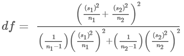
where C_level is 1 – α (2-tail test) or  1 - 2α (1-tail test)

 

8 Optional)

Use Confidence Interval With any C-level to test a claim or estimate mean differences  μ1 – μ2 or mean differences (\( \mu _d \) ).

 For  independent samples: Use Statdisk/Analysis /Confidence intervals/Mean two independent samples/

 For dependent samples: use Statdisk/Analysis/ Confidence intervals/Mean Match pairs

 Enter all inputs or data columns:

  Output:  Confidence interval:   L. limit < μ1 -  μ2 < U. limit, or

                                                L. limit < μ_d < U. limit and    p-value:

9) Make conclusion using C-level:

   i)  If the interval contains zero, conclude μ1 and μ2 have no significant difference. (L limit is negative U limit is positive.)

   ii) If the interval is all positive, conclude μ1 > μ2

       (L. Limit and U. Limits are both positive.)

   iii) If the interval is all negative, conclude μ1 < μ2.

       (L. limit and U. Limits are both negative.)

 

Note: When H0 is rejected, there is sufficient evidence to conclude that there is significant difference between μ1 and μ2.

 

Note: Conclusion from hypothesis test is exactly the same as the conclusion from Confidence Interval for testing of the mean because the standard errors are the same.

 

Ex1. A study claims that mean enrollment at two-year college is lower than at four-year colleges  in the United States. Two samples are collected, from the 35 two-year colleges surveyed, the mean enrollment was 5,068 with a standard deviation of 4,777. Of the 35 four-year colleges surveyed, the mean enrollment was 5,466 with a standard deviation of 8,191.  Test at sign. level of 0.05.

 

The samples are independent.

i) Define population 1 = two-year colleges, n1 = 35 \( \bar{x_1} \) = 5068, s1=4777, σ1 = not given,

  Define population 2 = four-year colleges, n2=35, \( \bar{x_2} \) = 5466, s2 = 8191, σ2 = not given.

ii) Claim: μ1 < μ2; H0 : μ1 = μ2;  Ha= μ1 < μ2

iii) Sign level = 0.05, left-tail test, use t-distribution.

iv) Use Statdisk/Analysis/Mean 2 independent samples

Select Alt. hypothesis : Pop Mean 1 < Pop Mean 2

Enter 0.05 to significance, enter n1 = 35, \( \bar{x_1} \) = 5068, s1=4777, σ1 = not given,

n2=35, \( \bar{x_2} \) = 5466 s2 = 8191, σ2 = not given. Use “Unequal variance, no Pool”. Evaluate.

Output  test stat t = -0.248, p-value = 0.4024

90% confidence interval = -3079.7 < μ1 – μ2 < 2283.7

v) since p-value (0.4024) > 0.05, fail to reject H0

vi) Since sample is not significant and the claim is Ha, the following statement is used for conclusion:

 There is not sufficient evidence to support the claim the mean enrollment in two-year college is less than those at four-year college.

 

 

Ex2. Use confidence interval at 95% confidence to estimate the difference in mean life of Duracell and Eveready battery. Sample results are as follow:

Duracell: n1 = 8, \( \bar{x_1} \) =41 hr, s1= 18 hr

Eveready: n2 = 10, \( \bar{x_2} \) = 45 hr, s2 = 20 hr

i) Samples are independent.

Define population 1 – Duracell

Define population 2 – Eveready

ii) Use Statdisk/Analysis/Confidence Intervals/

Mean 2 independent samples

Enter C-level = 0.95,

Enter sample 1 : n1 = 8, \( \bar{x_1} \) =41, s1= 18 hr

Enter sample 2: n2 = 10, \( \bar{x_2} \) = 45 hr, s2 = 20 hr

Use ‘Unequal variances, no Pool”. Evaluate

Output: p-value = 0.6618,  95% confidence interval

-23.05 <  µ1-µ2 < 15.05 hr

iii) Since zero contains in the interval, there is no sufficient evidence conclude there is significant difference.

Conclude that the mean life for the two batteries has no significant difference.

 

Ex3: A study of seat belt use involved children who were hospitalized after car accidents. For 123 children who were wearing seat belts, the number of days in ICU has a mean of 0.83 days and a standard deviation of 1.77 days. For the sample of 290 children who were not wearing seat belts, the number of days in ICU has a mean of 1.39 days and a standard deviation of 3.06 days. Test the claim at α = 0.05  by hypothesis and Confidence interval that seat belt use for children is effective in lowering the degree of injuries.

i) The two samples are independent. Values are summarized.

Define population 1: children who wear seat belts ,n1 = 123,   \( \bar{x_1} \) =0.83, s1=1.77

Define population 2: children who do not wear seat belts, n2 = 290,   \( \bar{x_1} \) =1.39, s1=3.06    

 ii)  Claim: μ1 < μ2, H0: μ1 =  μ2, Ha: μ1 < μ2

 iii) Use α = 0.05, left-tail test, use t distribution.

iv) Use Statdisk/Analysis/Hypothesis Testing /Mean 2 independent samples/

Select alternative hypothesis Mean 1 <  Mean 2

Enter significance = 0.05,

Enter  n1, \( \bar{x_1} \),  s1, n2, \( \bar{x_2} \),  s2.

Select options Unequal variances, no  pool.

Output: t = -2.33  p-value = 0.0102.

90% confidence interval is -0.9563< μ1 – μ2 < -0.1637

v) P-value (0.0102) < 0.05 Reject H0. There is significant difference between mean ICU times.

vi) There is sufficient evidence to support the claim that seat belt use for children is effective in lowering the degree of injuries.

 Confidence interval is -0.96 < μ1 -  μ2 < -0.16 days

 Since interval contains negative number, conclude there is sufficient evidence to show that μ1 <  μ2, so conclude degree of injuries for children wearing seat belts are lower.

Conclusion from hypothesis test and confidence interval are the same.

 

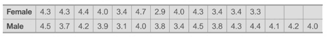
Ex4: Listed below are course evaluation scores for courses taught by female professors and male professors.

a) Use  \( \alpha \)= 0.05 to test the claim that there is a difference in mean evaluation scores of course taught by female professors and male professors.

i) The samples are independent because pairs of value are not matched or related.

Define population 1 – female professor scores

            population 2 – male professor scores

            Enter data to Statdisk.

ii) Claim: μ1 ≠  μ2, H0: μ1 =  μ2, Ha: μ1 ≠  μ2.

iii) Use α = 0.05, Two-tail test, use t distribution.

iv) Use Statdisk/Hypothesis Testing/Mean 2 independent samples / Click “use data” tab

Select “Population mean 1 not = pop mean 2” as alternative hypothesis, select columns for data, sample 1 is female professors’ scores,

sample 2 is male professors’ scores.

Use Unequal variances, No Pooled. Evaluate.

Output: t = -0.66, p-value(p) = 0.5172, df=19.06

Confidence interval (95%) -0.53 < μ1 - μ2 < 0.27.

v) p-value (0.5172 ) > 0.05, fail to reject H0. Conclude no significant difference.

vi) Since the claim is in H1: Conclusion about the claim: There is not sufficient evidence to support the claim that there is a difference in evaluation scores between course taught by female and male professor. Conclude plausibly no difference in scores.

 

vii) The confidence interval -0.53 < μ1 - μ2 < 0.27,   contains zero, conclude there could be no significant difference between the two means.  (Not sufficient evidence to support the claim of difference.

 

Ex5:  Assume Freshmen year for college student is from September to April of the following year. Use the sample data given below with a 0.05 significance level to test the claim that there is no difference(ie the same)  in mean weight change from September to April for students in their Freshman year. Samples are SRS and weights are normally distributed.

i) The samples are dependent because pairs of value are from the same student.

 define d = September weight – April weight

  Enter data to Statdisk.

ii) Claim: μ_d = 0,  H0: μ_d = 0,  H1: μ_d ≠0 (claim is H0)

iii) α= 0.05, two-tail test, use t -distribution.

iv) Use Statdisk/Analysis/Hypothesis Testings/Mean match pairs.

Select alt.  hypothesis: mean  of difference not =  0

Enter significance = 0.05,

Select sample 1 for September weights. Select Sample 2 for April's weights.  Evaluate.

Output t = -0.19, p-value(p) = 0.8605

95% confidence interval is -3.16 < \( \mu _d \) < 2.76 kg

v) P-value(0.8605) > 0.05, fail to reject H0.

vi) There is not sufficient evidence to reject the claim that there is no mean weight change from September to April for students in their freshmen year.

    Conclude the claim is plausibly true that there is no weights difference.

vii) Since Confidence interval is   -3.16 kg < \( \mu _d \)  < 2.76 kg. Interval contains zero. We are 95% confidence that the mean change in weight from September to April can be between an increase of 3.16 kg to a decrease of 2.76 kg.

Since the difference contains zero, conclude there is no mean difference at September and April’s weights.

Note: Conclusion from Hypothesis test and Confidence Interval are the same.

 

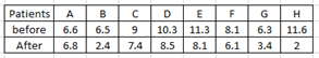
Ex 6: A study was conducted to investigate the effectiveness of hypnotism in reducing pain. Randomly selected subjects are given hypnotic treatment and their pain level before and after measured and recorded below.  Higher level corresponds to greater level of pain.

a) Conduct a hypothesis test to test the claim that hypnotism treatment can reduce pain. Use α= 0.05.

b) Construct an appropriate confidence interval for the mean difference of pain before and after hypnotism treatment.

i) The samples are dependent because each pair of values are from the same patient.

define d = before – after pain level.

 ( d > 0 if hypnotic treatment reduce pain)

Enter before and after data to Statdisk.

ii) Claim: μ_d > 0,  H0: μ_d = 0,  H1: μ_d > 0

iii) α= 0.05, two-tail test, use t -distribution

iv)  Use Statdisk/Analysis/Hypothesis Testing/Mean match pair.

Select alt. hypothesis : Mean of differences > 0 

Enter significance 0.05, select "before data" for sample 1, select after data for sample 2. Evaluate.

 Output:  \( \bar{d} \) = 3.125, sd= 2.91,  Output t = 3.04 and p-value = 0.0095

 90% confidence interval is 1.1748 <  μ_d <  5.0752

v) P-value (0.0095) < 0.05 reject H0.

vi) There is sufficient evidence to support the claim that hypnotism treatment can reduce pain level.

vii ) 90% Confidence interval is 1.17 <  μ_d < 5.08

Since the interval does not contain zero, there is a significant difference. The interval contains only positive values. So pain level before > pain level after.

Conclude hypnotism treatment can reduce pain.

Note: Conclusion from Hypothesis test and Confidence interval are the same.