
9.3: A Single Population Mean using the Normal Distribution
- Page ID
- 20074

All hypotheses tests have the same basic steps:
- Determine the hypothesis: What are we trying to figure out? This is formally written as the null and alternative hypotheses.
- The alternative hypothesis, \(H_{a}\), never has a symbol that contains an equal sign.
- The alternative hypothesis, \(H_{a}\), tells you if the test is left, right, or two-tailed. It is the key to conducting the appropriate test.
- Calculate the evidence: This will be a test statistics and either a critical value or a p-value.
- In a hypothesis test problem, you may see words such as "the level of significance is 1%." The "1%" is the preconceived or preset \(\alpha\). The statistician setting up the hypothesis test selects the value of α to use before collecting the sample data. If no level of significance is given, a common standard to use is \(\alpha = 0.05\).
- When you calculate the \(p\)-value and draw the picture, the \(p\)-value is the area in the left tail, the right tail, or split evenly between the two tails. For this reason, we call the hypothesis test left, right, or two tailed.
- Make a decision: The options will be Reject the Null Hypothesis or Do not Reject the Null Hypothesis.
- Never, ever, Accept the Null Hypothesis.
- Thinking about the meaning of the \(p\)-value: A data analyst (and anyone else) should have more confidence that he made the correct decision to reject the null hypothesis with a smaller \(p\)-value (for example, 0.001 as opposed to 0.04) even if using the 0.05 level for alpha. Similarly, for a large p-value such as 0.4, as opposed to a \(p\)-value of 0.056 (\(\alpha = 0.05\) is less than either number), a data analyst should have more confidence that she made the correct decision in not rejecting the null hypothesis. This makes the data analyst use judgment rather than mindlessly applying rules.
- Determine the conclusion: What does the decision mean in terms of the problem given?
Direction of Tail
\(H_{0}: \mu \geq 5, H_{a}: \mu < 5\)
Test of a single population mean. \(H_{a}\) tells you the test is left-tailed. The picture of the \(p\)-value is as follows:

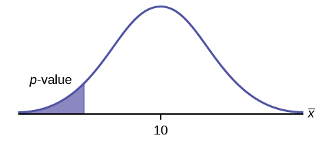
\(H_{0}: \mu \geq 10, H_{a}: \mu < 10\)
Assume the \(p\)-value is 0.0935. What type of test is this? Draw the picture of the \(p\)-value.
Answer
left-tailed test
\(H_{0}: \mu \leq 0.2, H_{a}: \mu > 0.2\)
This is a test of a single population proportion. \(H_{a}\) tells you the test is right-tailed. The picture of the p-value is as follows:

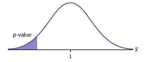
\(H_{0}: \mu \leq 1, H_{a}: \mu > 1\)
Assume the \(p\)-value is 0.1243. What type of test is this? Draw the picture of the \(p\)-value.
Answer
right-tailed test
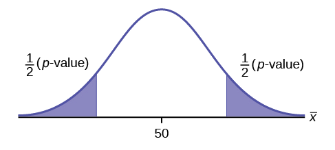
\(H_{0}: \mu = 50, H_{a}: \mu \neq 50\)
This is a test of a single population mean. \(H_{a}\) tells you the test is two-tailed. The picture of the \(p\)-value is as follows.
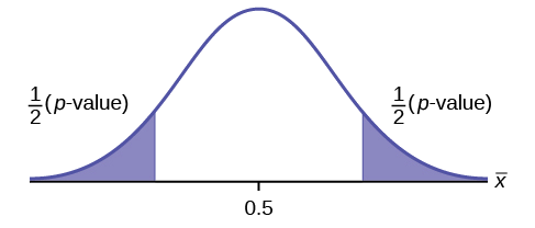
\(H_{0}: \mu = 0.5, H_{a}: \mu \neq 0.5\)
Assume the p-value is 0.2564. What type of test is this? Draw the picture of the \(p\)-value.
Answer
two-tailed test
Full Hypothesis Test Examples
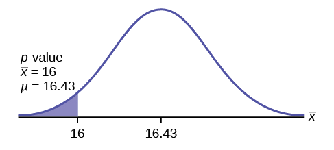
Jeffrey, as an eight-year old, established a mean time of 16.43 seconds for swimming the 25-yard freestyle, with a standard deviation of 0.8 seconds. His dad, Frank, thought that Jeffrey could swim the 25-yard freestyle faster using goggles. Frank bought Jeffrey a new pair of expensive goggles and timed Jeffrey for 15 25-yard freestyle swims. For the 15 swims, Jeffrey's mean time was 16 seconds. Frank thought that the goggles helped Jeffrey to swim faster than the 16.43 seconds. Conduct a hypothesis test using a preset α = 0.05. Assume that the swim times for the 25-yard freestyle are normal.
\(P\)-value Solution
Determine the hypothesis:
Since the problem is about a mean, this is a test of a single population mean.
For Jeffrey to swim faster, his time will be less than 16.43 seconds. So the claim will be that he can swim it in less time than 16.43 seconds.
\(H_{0}: \mu \geq 16.43\)
\(H_{a}: \mu < 16.43\) (claim)
The "\(<\)" in the alternative hypothesis tells you this is left-tailed.
Calculate the evidence:
Use the Standard Normal Distribution since the population standard deviation is given.
Calculate the test statistic using the same formula as a \(z\)-score using the Central Limit Theorem.
\[z=\frac{\bar{x}-\mu}{\frac{\sigma}{\sqrt{n}}}\nonumber\]
\(\mu = 16.43\) comes from \(H_{0}\) and not the data. \(\sigma = 0.8\) and \(n = 15\). Which gives
\[z=\frac{16-16.43}{\frac{0.8}{\sqrt{15}}}=\frac{-0.43}{\frac{0.8}{3.87298}}=\frac{-0.43}{0.20656}=-2.0817\nonumber\]
Now calculate the p-value based on the test statistic found.
This is a left-tailed test, so use the Excel formula \(=\text{NORM.S.DIST}(z,\text{true})\).
In this case, we found \(z\), which is the test statistic, to be \(z=-2.0817\).
Use the Excel formula \(=\text{NORM.S.DIST}(-2.0817,\text{true})=0.0187\).
So the \(p\text{-value} = 0.0187\). This is the area to the left of the sample mean, which is given as 16.
Make a decision:
Interpretation of the \(p-\text{value}\): If \(H_{0}\) is true, there is a 0.0187 probability (1.87%) that Jeffrey's mean time to swim the 25-yard freestyle is 16 seconds or less. Because a 1.87% chance is small, the mean time of 16 seconds or less is unlikely to have happened randomly. It is a rare event.
\(\mu = 16.43\) comes from \(H_{0}\). Our assumption gives \(\mu = 16.43\).
\(\alpha\) is the minimum area that could be considered to make our result significant.
Compare \(\alpha\) and the \(p\text{-value}\)
- If \(p\text{-value}\) is less than the \(\alpha\) then we will Reject \(H_0\).
- If \(\alpha\) is less than the \(p\text{-value}\) then we will Fail to Reject \(H_0\).
\(\alpha = 0.05\) and \(p\text{-value} = 0.0187\), so \(p\text{-value}<\alpha\)
Since \(p\text{-value}<\alpha\), reject \(H_{0}\).
Conclusion:
This means that you reject \(\mu \geq 16.43\).
There is sufficient evidence to support the claim that Jeffrey's mean swim time for the 25-yard freestyle is less than 16.43 seconds.
Critical Value Solution
Determine the hypothesis (Same as the \(P\)-value solution):
Since the problem is about a mean, this is a test of a single population mean.
For Jeffrey to swim faster, his time will be less than 16.43 seconds. So the claim will be that he can swim it in less time than 16.43 seconds.
\(H_{0}: \mu \geq 16.43\)
\(H_{a}: \mu < 16.43\) (claim)
The "\(<\)" in the alternative hypothesis tells you this is left-tailed.
Calculate the evidence:
Use the Standard Normal Distribution since the population standard deviation is given.
Calculate the critical value. Use the Standard Normal Distribution, Critical Value, Right-tail Excel formula: \(=\text{NORM.S.INV}(\alpha)\).
In this problem, the \(\alpha=0.05\), so use \(=\text{NORM.S.INV}(0.05)=-1.64485\)
Calculate the test statistic using the same formula as a \(z\)-score using the Central Limit Theorem.
\[z=\frac{\bar{x}-\mu}{\frac{\sigma}{\sqrt{n}}}\nonumber\]
\(\mu = 16.43\) comes from \(H_{0}\) and not the data. \(\sigma = 0.8\) and \(n = 15\). Which gives
\[z=\frac{16-16.43}{\frac{0.8}{\sqrt{15}}}=\frac{-0.43}{\frac{0.8}{3.87298}}=\frac{-0.43}{0.20656}=-2.0817\nonumber\]
Make a decision:
Graph the critical value and the test statistic along the number line of the Standard Normal Distribution graph.
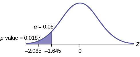
Since this is left-tailed, everything less than the critical value, \(\text{CV}=-1.64485\) will be the rejection region.
Since the test statistic, \(z=-2.0817\) is less than the critical value, \(\text{CV}=-1.64485, the decision will be to Reject the Null Hypothesis.
Conclusion (Same as the \(P\)-value solution):
This means that you reject \(\mu \geq 16.43\).
There is sufficient evidence to support the claim that Jeffrey's mean swim time for the 25-yard freestyle is less than 16.43 seconds.
The Type I and Type II errors for this problem are as follows:
The Type I error is to conclude that Jeffrey swims the 25-yard freestyle, on average, in less than 16.43 seconds when, in fact, he actually swims the 25-yard freestyle, on average, in 16.43 seconds. (Reject the null hypothesis when the null hypothesis is true.)
The Type II error is that there is not evidence to conclude that Jeffrey swims the 25-yard free-style, on average, in less than 16.43 seconds when, in fact, he actually does swim the 25-yard free-style, on average, in less than 16.43 seconds. (Do not reject the null hypothesis when the null hypothesis is false.)
The mean throwing distance of a football for a Marco, a high school freshman quarterback, is 40 yards, with a standard deviation of two yards. The team coach tells Marco to adjust his grip to get more distance. The coach records the distances for 20 throws. For the 20 throws, Marco’s mean distance was 45 yards. The coach thought the different grip helped Marco throw farther than 40 yards. Conduct a hypothesis test using a preset \(\alpha = 0.01\). Assume the throw distances for footballs are normal. Use the critical value method.
Answer
Determine the hypothesis:
Since the problem is about a mean, this is a test of a single population mean.
For Marco to throw farther, his distance will be greater than 40 yards. So the claim will be that he can throw farther than 40 yards.
\(H_{0}: \mu \leq 40\)
\(H_{a}: \mu > 40\) (claim)
The "\(>\)" in the alternative hypothesis tells you this is right-tailed.
Calculate the evidence:
Use the Standard Normal Distribution since the population standard deviation is given.
Calculate the critical value. Use the Standard Normal Distribution, Critical Value, Right-tail Excel formula: \(=\text{NORM.S.INV}(1-\alpha)\).
In this problem, the \(\alpha=0.01\), so use \(=\text{NORM.S.INV}(1-0.01)=2.3263\)
Calculate the test statistic using the same formula as a \(z\)-score using the Central Limit Theorem.
\[z=\frac{\bar{x}-\mu}{\frac{\sigma}{\sqrt{n}}}\nonumber\]
\(\mu = 40\) comes from \(H_{0}\) and not the data. \(\sigma = 2\) and \(n = 20\). Which gives
\[z=\frac{45-40}{\frac{2}{\sqrt{20}}}=\frac{5}{\frac{2}{4.4721}}=\frac{5}{0.4472}=11.1803\nonumber\]
Make a decision:
Graph the critical value and the test statistic along the number line of the Standard Normal Distribution graph.
Since this is right-tailed, everything greater than the critical value, \(\text{CV}=2.3263\) will be the rejection region.
Since the test statistic, \(z=11.1803\) is greater than the critical value, \(\text{CV}=2.3263\), the decision will be to Reject the Null Hypothesis.
Conclusion:
This means that you reject \(\mu \leq 40\).
There is sufficient evidence to support the claim that the change in Marco's grip improved his throwing distance to give a mean throw distance is greater than 40 yards.
A college football coach thought that his players could bench press a mean weight of 275 pounds. It is known that the standard deviation is 55 pounds. Three of his players thought that the mean weight was great than that amount. They asked 30 of their teammates for their estimated maximum lift on the bench press exercise. The data ranged from 205 pounds to 385 pounds. The actual different weights are given below
| 205 | 215 | 225 | 252 | 265 | 313 | 316 | 316 | 341 | 368 |
| 205 | 215 | 241 | 252 | 275 | 313 | 316 | 338 | 345 | 368 |
| 205 | 215 | 241 | 265 | 275 | 316 | 316 | 338 | 345 | 385 |
Conduct a \(p\)-value hypothesis test using a 2.5% level of significance to determine if the bench press mean is more than 275 pounds.
Answer
Determine the hypothesis:
Since the problem is about a mean weight, this is a test of a single population mean.
\(H_{0}: \mu \leq 275\)
\(H_{a}: \mu > 275\) (claim)
The "\(>\)" in the alternative hypothesis tells you this is a right-tailed test.
Calculate the evidence:
Use the Standard Normal Distribution since the population standard deviation is given.
Calculate the test statistic using the same formula as the \(z\)-score using the Central Limit Theorem.
\[z=\frac{\bar{x}-\mu}{\frac{\sigma}{\sqrt{n}}}\nonumber\]
\(\mu = 275\) comes from \(H_{0}\) and not the data. \(\sigma=55\) and \(n=30\). The problem does not give the sample mean, so that will need to be calculated using the data.
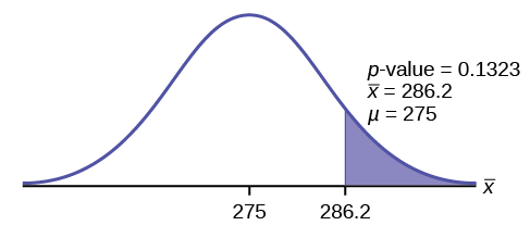
Enter the data into Excel, and use the Excel formula \(=\text{AVERAGE}()\) to find \(\bar{x}=286.2\).
\[z=\frac{286.2-275}{\frac{55}{\sqrt{30}}}=\frac{11.2}{\frac{2}{5.4772}}=\frac{11.2}{10.04}=1.11536\nonumber\]
Now calculate the \(p\)-value based on the test statistic found.
This is a right-tailed test, so use the Excel formula \(=1-\text{NORM.S.DIST}(z,\text{true})\).
In this case, we found \(z\), which is the test statistic, to be \(z=1.11536\).
Use the Excel formula \(=1-\text{NORM.S.DIST}(1.11536,\text{true})=0.132348\).
So the \(p\text{-value} = 0.132348\).
Interpretation of the p-value: If \(H_{0}\) is true, then there is a 0.1331 probability (13.23%) that the football players can lift a mean weight of 286.2 pounds or more. Because a 13.23% chance is large enough, a mean weight lift of 286.2 pounds or more is not a rare event.
Make a decision:
\(\alpha\) is the minimum area that could be considered to make our result significant.
Compare \(\alpha\) and the \(p\text{-value}\)
- If \(p\text{-value}\) is less than the \(\alpha\) then we will Reject \(H_0\).
- If \(\alpha\) is less than the \(p\text{-value}\) then we will Fail to Reject \(H_0\).
\(\alpha = 0.025\) and \(p\)-value \(= 0.1323\)
Since \(\alpha < p\text{-value}\), do not reject \(H_{0}\).
Conclusion: At the 2.5% level of significance, from the sample data, there is not sufficient evidence to conclude that the true mean weight lifted is more than 275 pounds.
Review
The hypothesis test itself has an established process. This can be summarized as follows:
- Determine \(H_{0}\) and \(H_{a}\). Remember, they are contradictory.
- Find the evidence: Draw a graph, calculate the test statistic, and use the test statistic to calculate the \(p\text{-value}\). (A z-score and a t-score are examples of test statistics.)
- Compare the preconceived α with the p-value, make a decision (reject or do not reject H0).
- Write a clear conclusion using English sentences.
Notice that in performing the hypothesis test, you use \(\alpha\) and not \(\beta\). \(\beta\) is needed to help determine the sample size of the data that is used in calculating the \(p\text{-value}\). Remember that the quantity \(1 – \beta\) is called the Power of the Test. A high power is desirable. If the power is too low, statisticians typically increase the sample size while keeping α the same.If the power is low, the null hypothesis might not be rejected when it should be.
Assume \(H_{0}: \mu = 9\) and \(H_{a}: \mu < 9\). Is this a left-tailed, right-tailed, or two-tailed test?
Answer
This is a left-tailed test.
Assume \(H_{0}: \mu \leq 6\) and \(H_{a}: \mu > 6\). Is this a left-tailed, right-tailed, or two-tailed test?
Assume \(H_{0}: p = 0.25\) and \(H_{a}: p \neq 0.25\). Is this a left-tailed, right-tailed, or two-tailed test?
Answer
This is a two-tailed test.
Draw the general graph of a left-tailed test.
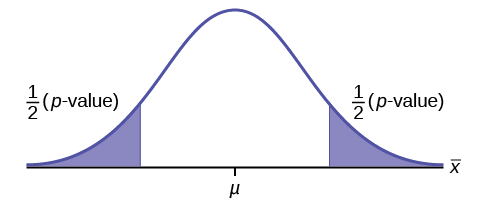
Draw the graph of a two-tailed test.
Answer
A bottle of water is labeled as containing 16 fluid ounces of water. You believe it is less than that. What type of test would you use?
Your friend claims that his mean golf score is 63. You want to show that it is higher than that. What type of test would you use?
Answer
a right-tailed test
A bathroom scale claims to be able to identify correctly any weight within a pound. You think that it cannot be that accurate. What type of test would you use?
You flip a coin and record whether it shows heads or tails. You know the probability of getting heads is 50%, but you think it is less for this particular coin. What type of test would you use?
Answer
a left-tailed test
If the alternative hypothesis has a not equals ( \(\neq\) ) symbol, you know to use which type of test?
Assume the null hypothesis states that the mean is at least 18. Is this a left-tailed, right-tailed, or two-tailed test?
Answer
This is a left-tailed test.
Assume the null hypothesis states that the mean is at most 12. Is this a left-tailed, right-tailed, or two-tailed test?
Assume the null hypothesis states that the mean is equal to 88. The alternative hypothesis states that the mean is not equal to 88. Is this a left-tailed, right-tailed, or two-tailed test?
Answer
This is a two-tailed test.
References
- Data from Amit Schitai. Director of Instructional Technology and Distance Learning. LBCC.
- Data from Bloomberg Businessweek. Available online at www.businessweek.com/news/2011- 09-15/nyc-smoking-rate-falls-to-record-low-of-14-bloomberg-says.html.
- Data from energy.gov. Available online at http://energy.gov (accessed June 27. 2013).
- Data from Gallup®. Available online at www.gallup.com (accessed June 27, 2013).
- Data from Growing by Degrees by Allen and Seaman.
- Data from La Leche League International. Available online at www.lalecheleague.org/Law/BAFeb01.html.
- Data from the American Automobile Association. Available online at www.aaa.com (accessed June 27, 2013).
- Data from the American Library Association. Available online at www.ala.org (accessed June 27, 2013).
- Data from the Bureau of Labor Statistics. Available online at http://www.bls.gov/oes/current/oes291111.htm.
- Data from the Centers for Disease Control and Prevention. Available online at www.cdc.gov (accessed June 27, 2013)
- Data from the U.S. Census Bureau, available online at quickfacts.census.gov/qfd/states/00000.html (accessed June 27, 2013).
- Data from the United States Census Bureau. Available online at www.census.gov/hhes/socdemo/language/.
- Data from Toastmasters International. Available online at http://toastmasters.org/artisan/deta...eID=429&Page=1.
- Data from Weather Underground. Available online at www.wunderground.com (accessed June 27, 2013).
- Federal Bureau of Investigations. “Uniform Crime Reports and Index of Crime in Daviess in the State of Kentucky enforced by Daviess County from 1985 to 2005.” Available online at http://www.disastercenter.com/kentucky/crime/3868.htm (accessed June 27, 2013).
- “Foothill-De Anza Community College District.” De Anza College, Winter 2006. Available online at research.fhda.edu/factbook/DA...t_da_2006w.pdf.
- Johansen, C., J. Boice, Jr., J. McLaughlin, J. Olsen. “Cellular Telephones and Cancer—a Nationwide Cohort Study in Denmark.” Institute of Cancer Epidemiology and the Danish Cancer Society, 93(3):203-7. Available online at http://www.ncbi.nlm.nih.gov/pubmed/11158188 (accessed June 27, 2013).
- Rape, Abuse & Incest National Network. “How often does sexual assault occur?” RAINN, 2009. Available online at www.rainn.org/get-information...sexual-assault (accessed June 27, 2013).
Glossary
- Central Limit Theorem
- Given a random variable (RV) with known mean \(\mu\) and known standard deviation \(\sigma\). We are sampling with size \(n\) and we are interested in two new RVs - the sample mean, \(\bar{X}\), and the sample sum, \(\sum X\). If the size \(n\) of the sample is sufficiently large, then \(\bar{X} - N\left(\mu, \frac{\sigma}{\sqrt{n}}\right)\) and \(\sum X - N \left(n\mu, \sqrt{n}\sigma\right)\). If the size n of the sample is sufficiently large, then the distribution of the sample means and the distribution of the sample sums will approximate a normal distribution regardless of the shape of the population. The mean of the sample means will equal the population mean and the mean of the sample sums will equal \(n\) times the population mean. The standard deviation of the distribution of the sample means, \(\frac{\sigma}{\sqrt{n}}\), is called the standard error of the mean.
Contributors and Attributions
Barbara Illowsky and Susan Dean (De Anza College) with many other contributing authors. Content produced by OpenStax College is licensed under a Creative Commons Attribution License 4.0 license. Download for free at http://cnx.org/contents/30189442-699...b91b9de@18.114.