9.2: Hypothesis Testing

All hypotheses tests have the same basic steps:

1. Determine the hypothesis: What are we trying to figure out? This is formally written as the null and alternative hypotheses.
2. Calculate the evidence: This will be a test statistics and either a critical value or a p-value.
3. Make a decision: The options will be Reject the Null Hypothesis or Do not Reject the Null Hypothesis.
4. Determine the conclusion: What does the decision mean in terms of the problem given?

Null and Alternative Hypotheses

The actual test begins by considering two hypotheses. They are called the null hypothesis and the alternative hypothesis. These hypotheses contain opposing viewpoints.

\(H_0\): The null hypothesis: It is a statement of no difference between the variables—they are not related. This can often be considered the status quo and as a result if you cannot accept the null it requires some action.

\(H_a\): The alternative hypothesis: It is a claim about the population that is contradictory to \(H_0\) and what we conclude when we reject \(H_0\). This is usually what the researcher is trying to prove.

Since the null and alternative hypotheses are contradictory, you must examine evidence to decide if you have enough evidence to reject the null hypothesis or not. The evidence is in the form of sample data.

After you have determined which hypothesis the sample supports, you make a decision. There are two options for a decision. They are "reject \(H_0\)" if the sample information favors the alternative hypothesis or "do not reject \(H_0\)" or "decline to reject \(H_0\)" if the sample information is insufficient to reject the null hypothesis.

Table \(\PageIndex{1}\): Mathematical Symbols Used in \(H_{0}\) and \(H_{a}\):

\(H_{0}\)	\(H_{a}\)
equal (=)	not equal \((\neq)\) or greater than (>) or less than (<)
greater than or equal to \((\geq)\)	less than (<)
less than or equal to \((\geq)\)	more than (>)

\(H_{0}\) always has a symbol with an equal in it. \(H_{a}\) never has a symbol with an equal in it. The choice of symbol depends on the wording of the hypothesis test. However, be aware that many researchers (including one of the co-authors in research work) use = in the null hypothesis, even with > or < as the symbol in the alternative hypothesis. This practice is acceptable because we only make the decision to reject or not reject the null hypothesis.

Example \(\PageIndex{1}\)

• \(H_{0}\): No more than 30% of the registered voters in Santa Clara County voted in the primary election. \(p \leq 30\)
• \(H_{a}\): More than 30% of the registered voters in Santa Clara County voted in the primary election. \(p > 30\)

Exercise \(\PageIndex{1}\)

A medical trial is conducted to test whether or not a new medicine reduces cholesterol by 25%. State the null and alternative hypotheses.

Answer

• \(H_{0}\): The drug reduces cholesterol by 25%. \(p = 0.25\)
• \(H_{a}\): The drug does not reduce cholesterol by 25%. \(p \neq 0.25\)

Example \(\PageIndex{2}\)

We want to test whether the mean GPA of students in American colleges is different from 2.0 (out of 4.0). The null and alternative hypotheses are:

• \(H_{0}: \mu = 2.0\)
• \(H_{a}: \mu \neq 2.0\)

Exercise \(\PageIndex{2}\)

We want to test whether the mean height of eighth graders is 66 inches. State the null and alternative hypotheses. Fill in the correct symbol \((=, \neq, \geq, <, \leq, >)\) for the null and alternative hypotheses.

• \(H_{0}: \mu_ 66\)
• \(H_{a}: \mu_ 66\)

Answer

• \(H_{0}: \mu = 66\)
• \(H_{a}: \mu \neq 66\)

Example \(\PageIndex{3}\)

We want to test if college students take less than five years to graduate from college, on the average. The null and alternative hypotheses are:

• \(H_{0}: \mu \geq 66\)
• \(H_{a}: \mu < 66\)

Exercise \(\PageIndex{3}\)

We want to test if it takes fewer than 45 minutes to teach a lesson plan. State the null and alternative hypotheses. Fill in the correct symbol ( =, ≠, ≥, <, ≤, >) for the null and alternative hypotheses.

1. \(H_{0}: \mu_ 45\)
2. \(H_{a}: \mu_ 45\)

Answer

1. \(H_{0}: \mu \geq 45\)
2. \(H_{a}: \mu < 45\)

Example \(\PageIndex{4}\)

In an issue of U. S. News and World Report, an article on school standards stated that about half of all students in France, Germany, and Israel take advanced placement exams and a third pass. The same article stated that 6.6% of U.S. students take advanced placement exams and 4.4% pass. Test if the percentage of U.S. students who take advanced placement exams is more than 6.6%. State the null and alternative hypotheses.

• \(H_{0}: p \leq 0.066\)
• \(H_{a}: p > 0.066\)

Exercise \(\PageIndex{4}\)

On a state driver’s test, about 40% pass the test on the first try. We want to test if more than 40% pass on the first try. Fill in the correct symbol (\(=, \neq, \geq, <, \leq, >\)) for the null and alternative hypotheses.

1. \(H_{0}: p_ 0.40\)
2. \(H_{a}: p_ 0.40\)

Answer

1. \(H_{0}: p = 0.40\)
2. \(H_{a}: p > 0.40\)

COLLABORATIVE EXERCISE

Bring to class a newspaper, some news magazines, and some Internet articles . In groups, find articles from which your group can write null and alternative hypotheses. Discuss your hypotheses with the rest of the class.

Outcomes and the Type I and Type II Errors

When you perform a hypothesis test, there are four possible outcomes depending on the actual truth (or falseness) of the null hypothesis \(H_{0}\) and the decision to reject or not. The outcomes are summarized in the following table:

ACTION	\(H_{0}\) is Actually True	\(H_{0}\) is Actually False
Do not reject \(H_{0}\)	Correct Outcome	Type II error
Reject \(H_{0}\)	Type I Error	Correct Outcome

The four possible outcomes in the table are:

1. The decision is not to reject \(H_{0}\) when \(H_{0}\) is true (correct decision).
2. The decision is to reject \(H_{0}\) when \(H_{0}\) is true (incorrect decision known as aType I error).
3. The decision is not to reject \(H_{0}\) when, in fact, \(H_{0}\) is false (incorrect decision known as a Type II error).
4. The decision is to reject \(H_{0}\) when \(H_{0}\) is false (correct decision whose probability is called the Power of the Test).

Each of the errors occurs with a particular probability. The Greek letters \(\alpha\) and \(\beta\) represent the probabilities.

• \(\alpha =\) probability of a Type I error \(= P(\text{Type I error}) =\) probability of rejecting the null hypothesis when the null hypothesis is true.
• \(\beta =\) probability of a Type II error \(= P(\text{Type II error}) =\) probability of not rejecting the null hypothesis when the null hypothesis is false.

\(\alpha\) and \(\beta\) should be as small as possible because they are probabilities of errors. They are rarely zero.

The Power of the Test is \(1 - \beta\). Ideally, we want a high power that is as close to one as possible. Increasing the sample size can increase the Power of the Test. The following are examples of Type I and Type II errors.

Example \(\PageIndex{5}\): Type I vs. Type II errors

Suppose the null hypothesis, \(H_{0}\), is: Frank's rock climbing equipment is safe.

• Type I error: Frank thinks that his rock climbing equipment may not be safe when, in fact, it really is safe.
• Type II error: Frank thinks that his rock climbing equipment may be safe when, in fact, it is not safe.

\(\alpha =\) probability that Frank thinks his rock climbing equipment may not be safe when, in fact, it really is safe.

\(\beta =\) probability that Frank thinks his rock climbing equipment may be safe when, in fact, it is not safe.

Notice that, in this case, the error with the greater consequence is the Type II error. (If Frank thinks his rock climbing equipment is safe, he will go ahead and use it.)

Exercise \(\PageIndex{5}\)

Suppose the null hypothesis, \(H_{0}\), is: the blood cultures contain no traces of pathogen \(X\). State the Type I and Type II errors.

Answer

• Type I error: The researcher thinks the blood cultures do contain traces of pathogen \(X\), when in fact, they do not.
• Type II error: The researcher thinks the blood cultures do not contain traces of pathogen \(X\), when in fact, they do.

Example \(\PageIndex{6}\)

Suppose the null hypothesis, \(H_{0}\), is: The victim of an automobile accident is alive when he arrives at the emergency room of a hospital.

• Type I error: The emergency crew thinks that the victim is dead when, in fact, the victim is alive.
• Type II error: The emergency crew does not know if the victim is alive when, in fact, the victim is dead.

\(\alpha =\) probability that the emergency crew thinks the victim is dead when, in fact, he is really alive \(= P(\text{Type I error})\).

\(\beta =\) probability that the emergency crew does not know if the victim is alive when, in fact, the victim is dead \(= P(\text{Type II error})\).

The error with the greater consequence is the Type I error. (If the emergency crew thinks the victim is dead, they will not treat him.)

Exercise \(\PageIndex{6}\)

Suppose the null hypothesis, \(H_{0}\), is: a patient is not sick. Which type of error has the greater consequence, Type I or Type II?

Answer

The error with the greater consequence is the Type II error: the patient will be thought well when, in fact, he is sick, so he will not get treatment.

Example \(\PageIndex{7}\)

It’s a Boy Genetic Labs claim to be able to increase the likelihood that a pregnancy will result in a boy being born. Statisticians want to test the claim. Suppose that the null hypothesis, \(H_{0}\), is: It’s a Boy Genetic Labs has no effect on gender outcome.

• Type I error: This results when a true null hypothesis is rejected. In the context of this scenario, we would state that we believe that It’s a Boy Genetic Labs influences the gender outcome, when in fact it has no effect. The probability of this error occurring is denoted by the Greek letter alpha, \(\alpha\).
• Type II error: This results when we fail to reject a false null hypothesis. In context, we would state that It’s a Boy Genetic Labs does not influence the gender outcome of a pregnancy when, in fact, it does. The probability of this error occurring is denoted by the Greek letter beta, \(\beta\).

The error of greater consequence would be the Type I error since couples would use the It’s a Boy Genetic Labs product in hopes of increasing the chances of having a boy.

Exercise \(\PageIndex{7}\)

“Red tide” is a bloom of poison-producing algae–a few different species of a class of plankton called dinoflagellates. When the weather and water conditions cause these blooms, shellfish such as clams living in the area develop dangerous levels of a paralysis-inducing toxin. In Massachusetts, the Division of Marine Fisheries (DMF) monitors levels of the toxin in shellfish by regular sampling of shellfish along the coastline. If the mean level of toxin in clams exceeds 800 μg (micrograms) of toxin per kg of clam meat in any area, clam harvesting is banned there until the bloom is over and levels of toxin in clams subside. Describe both a Type I and a Type II error in this context, and state which error has the greater consequence.

Answer

In this scenario, an appropriate null hypothesis would be \(H_{0}\): the mean level of toxins is at most \(800 \mu\text{g}\), \(H_{0}: \mu_{0} \leq 800 \mu\text{g}\).

Type I error: The DMF believes that toxin levels are still too high when, in fact, toxin levels are at most \(800 \mu\text{g}\). The DMF continues the harvesting ban.

Type II error: The DMF believes that toxin levels are within acceptable levels (are at least 800 μg) when, in fact, toxin levels are still too high (more than \(800 \mu\text{g}\)). The DMF lifts the harvesting ban. This error could be the most serious. If the ban is lifted and clams are still toxic, consumers could possibly eat tainted food.

In summary, the more dangerous error would be to commit a Type II error, because this error involves the availability of tainted clams for consumption.

Example \(\PageIndex{8}\)

A certain experimental drug claims a cure rate of at least 75% for males with prostate cancer. Describe both the Type I and Type II errors in context. Which error is the more serious?

• Type I: A cancer patient believes the cure rate for the drug is less than 75% when it actually is at least 75%.
• Type II: A cancer patient believes the experimental drug has at least a 75% cure rate when it has a cure rate that is less than 75%.

In this scenario, the Type II error contains the more severe consequence. If a patient believes the drug works at least 75% of the time, this most likely will influence the patient’s (and doctor’s) choice about whether to use the drug as a treatment option.

Exercise \(\PageIndex{8}\)

Determine both Type I and Type II errors for the following scenario:

Assume a null hypothesis, \(H_{0}\), that states the percentage of adults with jobs is at least 88%. Identify the Type I and Type II errors from these four statements.

1. Not to reject the null hypothesis that the percentage of adults who have jobs is at least 88% when that percentage is actually less than 88%
2. Not to reject the null hypothesis that the percentage of adults who have jobs is at least 88% when the percentage is actually at least 88%.
3. Reject the null hypothesis that the percentage of adults who have jobs is at least 88% when the percentage is actually at least 88%.
4. Reject the null hypothesis that the percentage of adults who have jobs is at least 88% when that percentage is actually less than 88%.

Answer

Type I error: c

Type I error: b

Distribution Needed for Hypothesis Testing

Earlier in the course, we discussed sampling distributions. Particular distributions are associated with hypothesis testing. Perform tests of a population mean using a normal distribution or a Student's \(t\)-distribution. (Remember, use a Student's \(t\)-distribution when the population standard deviation is unknown and the distribution of the sample mean is approximately normal.) We perform tests of a population proportion using a normal distribution (usually \(n\) is large or the sample size is large).

If you are testing a single population mean, the distribution for the test is for means:

\[\bar{X} - N\left(\mu_{x}, \frac{\sigma_{x}}{\sqrt{n}}\right)\]

or

\[t_{df}\]

The population parameter is \(\mu\). The estimated value (point estimate) for \(\mu\) is \(\bar{x}\), the sample mean.

If you are testing a single population proportion, the distribution for the test is for proportions or percentages:

\[P' - N\left(p, \sqrt{\frac{p-q}{n}}\right)\]

The population parameter is \(p\). The estimated value (point estimate) for \(p\) is \(p′\). \(p' = \frac{x}{n}\) where \(x\) is the number of successes and n is the sample size.

Assumptions

When you perform a hypothesis test of a single population mean \(\mu\) using a Student's \(t\)-distribution (often called a \(t\)-test), there are fundamental assumptions that need to be met in order for the test to work properly. Your data should be a simple random sample that comes from a population that is approximately normally distributed. You use the sample standard deviation to approximate the population standard deviation. (Note that if the sample size is sufficiently large, a \(t\)-test will work even if the population is not approximately normally distributed).

When you perform a hypothesis test of a single population mean \(\mu\) using a normal distribution (often called a \(z\)-test), you take a simple random sample from the population. The population you are testing is normally distributed or your sample size is sufficiently large. You know the value of the population standard deviation which, in reality, is rarely known.

When you perform a hypothesis test of a single population proportion \(p\), you take a simple random sample from the population. You must meet the conditions for a binomial distribution which are: there are a certain number \(n\) of independent trials, the outcomes of any trial are success or failure, and each trial has the same probability of a success \(p\). The shape of the binomial distribution needs to be similar to the shape of the normal distribution. To ensure this, the quantities \(np\) and \(nq\) must both be greater than five \((np > 5\) and \(nq > 5)\). Then the binomial distribution of a sample (estimated) proportion can be approximated by the normal distribution with \(\mu = p\) and \(\sigma = \sqrt{\frac{pq}{n}}\). Remember that \(q = 1 – p\).

Rare Events, the Sample, Decision and Conclusion

Establishing the type of distribution, sample size, and known or unknown standard deviation can help you figure out how to go about a hypothesis test. However, there are several other factors you should consider when working out a hypothesis test.

Rare Events

Suppose you make an assumption about a property of the population (this assumption is the null hypothesis). Then you gather sample data randomly. If the sample has properties that would be very unlikely to occur if the assumption is true, then you would conclude that your assumption about the population is probably incorrect. (Remember that your assumption is just an assumption—it is not a fact and it may or may not be true. But your sample data are real and the data are showing you a fact that seems to contradict your assumption.)

For example, Didi and Ali are at a birthday party of a very wealthy friend. They hurry to be first in line to grab a prize from a tall basket that they cannot see inside because they will be blindfolded. There are 200 plastic bubbles in the basket and Didi and Ali have been told that there is only one with a $100 bill. Didi is the first person to reach into the basket and pull out a bubble. Her bubble contains a $100 bill. The probability of this happening is \(\frac{1}{200} = 0.005\). Because this is so unlikely, Ali is hoping that what the two of them were told is wrong and there are more $100 bills in the basket. A "rare event" has occurred (Didi getting the $100 bill) so Ali doubts the assumption about only one $100 bill being in the basket.

Using the Sample to Test the Null Hypothesis

Use the sample data to calculate the actual probability of getting the test result, called the \(p\)-value. The \(p\)-value is the probability that, if the null hypothesis is true, the results from another randomly selected sample will be as extreme or more extreme as the results obtained from the given sample.

A large \(p\)-value calculated from the data indicates that we should not reject the null hypothesis. The smaller the \(p\)-value, the more unlikely the outcome, and the stronger the evidence is against the null hypothesis. We would reject the null hypothesis if the evidence is strongly against it.

Draw a graph that shows the \(p\)-value. The hypothesis test is easier to perform if you use a graph because you see the problem more clearly.

Example \(\PageIndex{9}\)

Suppose a baker claims that his bread height is more than 15 cm, on average. Several of his customers do not believe him. To persuade his customers that he is right, the baker decides to do a hypothesis test. He bakes 10 loaves of bread. The mean height of the sample loaves is 17 cm. The baker knows from baking hundreds of loaves of bread that the standard deviation for the height is 0.5 cm. and the distribution of heights is normal.

• The null hypothesis could be \(H_{0}: \mu \leq 15\)
• The alternate hypothesis is \(H_{a}: \mu > 15\)

The words "is more than" translates as a "\(>\)" so "\(\mu > 15\)" goes into the alternate hypothesis. The null hypothesis must contradict the alternate hypothesis.

Since \(\sigma\) is known (\(\sigma = 0.5 cm.\)), the distribution for the population is known to be normal with mean \(μ = 15\) and standard deviation

\[\dfrac{\sigma}{\sqrt{n}} = \frac{0.5}{\sqrt{10}} = 0.16. \nonumber\]

Suppose the null hypothesis is true (the mean height of the loaves is no more than 15 cm). Then is the mean height (17 cm) calculated from the sample unexpectedly large? The hypothesis test works by asking the question how unlikely the sample mean would be if the null hypothesis were true. The graph shows how far out the sample mean is on the normal curve. The p-value is the probability that, if we were to take other samples, any other sample mean would fall at least as far out as 17 cm.

The \(p\)-value, then, is the probability that a sample mean is the same or greater than 17 cm. when the population mean is, in fact, 15 cm. We can calculate this probability using the normal distribution for means.

Figure \(\PageIndex{1}\)

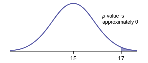
\(p\text{-value} = P(\bar{x} > 17)\) which is approximately zero.

A \(p\)-value of approximately zero tells us that it is highly unlikely that a loaf of bread rises no more than 15 cm, on average. That is, almost 0% of all loaves of bread would be at least as high as 17 cm. purely by CHANCE had the population mean height really been 15 cm. Because the outcome of 17 cm. is so unlikely (meaning it is happening NOT by chance alone), we conclude that the evidence is strongly against the null hypothesis (the mean height is at most 15 cm.). There is sufficient evidence that the true mean height for the population of the baker's loaves of bread is greater than 15 cm.

Exercise \(\PageIndex{9}\)

A normal distribution has a standard deviation of 1. We want to verify a claim that the mean is greater than 12. A sample of 36 is taken with a sample mean of 12.5.

• \(H_{0}: \mu leq 12\)
• \(H_{a}: \mu > 12\)

The \(p\)-value is 0.0013

Draw a graph that shows the \(p\)-value.

Answer

\(p\text{-value} = 0.0013\)

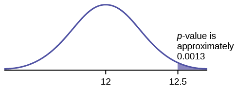
Figure \(\PageIndex{2}\)

Decision and Conclusion

A systematic way to make a decision of whether to reject or not reject the null hypothesis is to compare the \(p\)-value and a preset or preconceived \(\alpha\) (also called a "significance level"). A preset \(\alpha\) is the probability of a Type I error (rejecting the null hypothesis when the null hypothesis is true). It may or may not be given to you at the beginning of the problem.

When you make a decision to reject or not reject \(H_{0}\), do as follows:

• If \(\alpha > p\text{-value}\), reject \(H_{0}\). The results of the sample data are significant. There is sufficient evidence to conclude that \(H_{0}\) is an incorrect belief and that the alternative hypothesis, \(H_{a}\), may be correct.
• If \(\alpha \leq p\text{-value}\), do not reject \(H_{0}\). The results of the sample data are not significant.There is not sufficient evidence to conclude that the alternative hypothesis,\(H_{a}\), may be correct.

When you "do not reject \(H_{0}\)", it does not mean that you should believe that H₀ is true. It simply means that the sample data have failed to provide sufficient evidence to cast serious doubt about the truthfulness of \(H_{0}\).

Conclusion: After you make your decision, write a thoughtful conclusion about the hypotheses in terms of the given problem.

Example \(\PageIndex{10}\)

When using the \(p\)-value to evaluate a hypothesis test, it is sometimes useful to use the following memory device

• If the \(p\)-value is low, the null must go.
• If the \(p\)-value is high, the null must fly.

This memory aid relates a \(p\)-value less than the established alpha (the \(p\) is low) as rejecting the null hypothesis and, likewise, relates a \(p\)-value higher than the established alpha (the \(p\) is high) as not rejecting the null hypothesis.

Fill in the blanks.

Reject the null hypothesis when ______________________________________.

The results of the sample data _____________________________________.

Do not reject the null when hypothesis when __________________________________________.

The results of the sample data ____________________________________________.

Answer

Reject the null hypothesis when the \(p\)-value is less than the established alpha value. The results of the sample data support the alternative hypothesis.

Do not reject the null hypothesis when the \(p\)-value is greater than the established alpha value. The results of the sample data do not support the alternative hypothesis.

Exercise \(\PageIndex{10}\)

It’s a Boy Genetics Labs claim their procedures improve the chances of a boy being born. The results for a test of a single population proportion are as follows:

• \(H_{0}: p = 0.50, H_{a}: p > 0.50\)
• \(\alpha = 0.01\)
• \(p\text{-value} = 0.025\)

Interpret the results and state a conclusion in simple, non-technical terms.

Answer

Since the \(p\)-value is greater than the established alpha value (the \(p\)-value is high), we do not reject the null hypothesis. There is not enough evidence to support It’s a Boy Genetics Labs' stated claim that their procedures improve the chances of a boy being born.

Review

Null and Alternative Hypotheses

In a hypothesis test, sample data is evaluated in order to arrive at a decision about some type of claim. If certain conditions about the sample are satisfied, then the claim can be evaluated for a population. In a hypothesis test, we:

1. Evaluate the null hypothesis, typically denoted with \(H_{0}\). The null is not rejected unless the hypothesis test shows otherwise. The null statement must always contain some form of equality \((=, \leq \text{or} \geq)\)
2. Always write the alternative hypothesis, typically denoted with \(H_{a}\) or \(H_{1}\), using less than, greater than, or not equals symbols, i.e., \((\neq, >, \text{or} <)\).
3. If we reject the null hypothesis, then we can assume there is enough evidence to support the alternative hypothesis.
4. Never state that a claim is proven true or false. Keep in mind the underlying fact that hypothesis testing is based on probability laws; therefore, we can talk only in terms of non-absolute certainties.

Outcomes and the Type I and Type II Errors

In every hypothesis test, the outcomes are dependent on a correct interpretation of the data. Incorrect calculations or misunderstood summary statistics can yield errors that affect the results. A Type I error occurs when a true null hypothesis is rejected. A Type II error occurs when a false null hypothesis is not rejected. The probabilities of these errors are denoted by the Greek letters \(\alpha\) and \(\beta\), for a Type I and a Type II error respectively. The power of the test, \(1 - \beta\), quantifies the likelihood that a test will yield the correct result of a true alternative hypothesis being accepted. A high power is desirable.

Distribution Needed for Hypothesis Testing

In order for a hypothesis test’s results to be generalized to a population, certain requirements must be satisfied.

When testing for a single population mean:

1. A Student's \(t\)-test should be used if the data come from a simple, random sample and the population is approximately normally distributed, or the sample size is large, with an unknown standard deviation.
2. The normal test will work if the data come from a simple, random sample and the population is approximately normally distributed, or the sample size is large, with a known standard deviation.

When testing a single population proportion use a normal test for a single population proportion if the data comes from a simple, random sample, fill the requirements for a binomial distribution, and the mean number of successes and the mean number of failures satisfy the conditions: \(np > 5\) and \(nq > 5\) where \(n\) is the sample size, \(p\) is the probability of a success, and \(q\) is the probability of a failure.

Rare Events, the Sample, Decision and Conclusion

When the probability of an event occurring is low, and it happens, it is called a rare event. Rare events are important to consider in hypothesis testing because they can inform your willingness not to reject or to reject a null hypothesis. To test a null hypothesis, find the p-value for the sample data and graph the results. When deciding whether or not to reject the null the hypothesis, keep these two parameters in mind:

• \(\alpha > p-value\), reject the null hypothesis
• \(\alpha \leq p-value\), do not reject the null hypothesis

Formula Review

\(H_{0}\) and \(H_{a}\) are contradictory.

If \(H_{a}\) has:	equal \((=)\)	greater than or equal to \((\geq)\)	less than or equal to \((\leq)\)
then \(H_{a}\) has:	not equal \((\neq)\) or greater than \((>)\) or less than \((<)\)	less than \((<)\)	greater than \((>)\)

• If \(\alpha \leq p\)-value, then do not reject \(H_{0}\).
• If\(\alpha > p\)-value, then reject \(H_{0}\).

\(\alpha\) is preconceived. Its value is set before the hypothesis test starts. The \(p\)-value is calculated from the data.

• \(\alpha =\) probability of a Type I error \(= P(\text{Type I error}) =\) probability of rejecting the null hypothesis when the null hypothesis is true.
• \(\beta =\) probability of a Type II error \(= P(\text{Type II error}) =\) probability of not rejecting the null hypothesis when the null hypothesis is false.

If there is no given preconceived \(\alpha\), then use \(\alpha = 0.05\).

Types of Hypothesis Tests

• Single population mean, known population variance (or standard deviation): Normal test.
• Single population mean, unknown population variance (or standard deviation): Student's \(t\)-test.
• Single population proportion: Normal test.
• For a single population mean, we may use a normal distribution with the following mean and standard deviation. Means: \(\mu = \mu_{\bar{x}}\) and \(\\sigma_{\bar{x}} = \frac{\sigma_{x}}{\sqrt{n}}\)
• A single population proportion, we may use a normal distribution with the following mean and standard deviation. Proportions: \(\mu = p\) and \(\sigma = \sqrt{\frac{pq}{n}}\).

References

Data from the National Institute of Mental Health. Available online at http://www.nimh.nih.gov/publicat/depression.cfm.

Glossary

Hypothesis

a statement about the value of a population parameter, in case of two hypotheses, the statement assumed to be true is called the null hypothesis (notation \(H_{0}\)) and the contradictory statement is called the alternative hypothesis (notation \(H_{a}\)).

Type 1 Error

The decision is to reject the null hypothesis when, in fact, the null hypothesis is true.

Type 2 Error

The decision is not to reject the null hypothesis when, in fact, the null hypothesis is false.

Binomial Distribution

a discrete random variable (RV) that arises from Bernoulli trials. There are a fixed number, \(n\), of independent trials. “Independent” means that the result of any trial (for example, trial 1) does not affect the results of the following trials, and all trials are conducted under the same conditions. Under these circumstances the binomial RV Χ is defined as the number of successes in \(n\) trials. The notation is: \(X \sim B(n, p) \mu = np\) and the standard deviation is \(\sigma = \sqrt{npq}\). The probability of exactly \(x\) successes in \(n\) trials is \(P(X = x) = \binom{n}{x} p^{x}q^{n-x}\).

Normal Distribution

a continuous random variable (RV) with pdf \(f(x) = \frac{1}{\sigma\sqrt{2\pi}}e^{\frac{-(x-\mu)^{2}}{2\sigma^{2}}}\), where \(\mu\) is the mean of the distribution, and \(\sigma\) is the standard deviation, notation: \(X \sim N(\mu, \sigma)\). If \(\mu = 0\) and \(\sigma = 1\), the RV is called the standard normal distribution.

Standard Deviation

a number that is equal to the square root of the variance and measures how far data values are from their mean; notation: \(s\) for sample standard deviation and \(\sigma\) for population standard deviation.

Student's t-Distribution

investigated and reported by William S. Gossett in 1908 and published under the pseudonym Student. The major characteristics of the random variable (RV) are:

• It is continuous and assumes any real values.
• The pdf is symmetrical about its mean of zero. However, it is more spread out and flatter at the apex than the normal distribution.
• It approaches the standard normal distribution as \(n\) gets larger.
• There is a "family" of \(t\)-distributions: every representative of the family is completely defined by the number of degrees of freedom which is one less than the number of data items.

Level of Significance of the Test

probability of a Type I error (reject the null hypothesis when it is true). Notation: \(\alpha\). In hypothesis testing, the Level of Significance is called the preconceived \(\alpha\) or the preset \(\alpha\).

\(p\)-value

the probability that an event will happen purely by chance assuming the null hypothesis is true. The smaller the \(p\)-value, the stronger the evidence is against the null hypothesis.

Contributors and Attributions

• Barbara Illowsky and Susan Dean (De Anza College) with many other contributing authors. Content produced by OpenStax College is licensed under a Creative Commons Attribution License 4.0 license. Download for free at http://cnx.org/contents/30189442-699...b91b9de@18.114.