1.3: Eliminating Trend Components

In this section three different methods are developed to estimate the trend of a time series model. It is assumed that it makes sense to postulate the model (1.1.1) with \(s_t=0\) for all \(t\in T\), that is,

\[X_t=m_t+Y_t, t\in T \tag{1.3.1} \label{Eq131} \]

where (without loss of generality) \(E[Y_t]=0\). In particular, three different methods are discussed, (1) the least squares estimation of \(m_t\), (2) smoothing by means of moving averages and (3) differencing.

Method 1 (Least squares estimation) It is often useful to assume that a trend component can be modeled appropriately by a polynomial,

\[ m_t=b_0+b_1t+\ldots+b_pt^p, \qquad p\in\mathbb{N}_0. \nonumber \]

In this case, the unknown parameters \(b_0,\ldots,b_p\) can be estimated by the least squares method. Combined, they yield the estimated polynomial trend

\[ \hat{m}_t=\hat{b}_0+\hat{b}_1t+\ldots+\hat{b}_pt^p, \qquad t\in T, \nonumber \]

where \(\hat{b}_0,\ldots,\hat{b}_p\) denote the corresponding least squares estimates. Note that the order \(p\) is not estimated. It has to be selected by the statistician---for example, by inspecting the time series plot. The residuals \(\hat{Y}_t\) can be obtained as

\[ \hat{Y}_t=X_t-\hat{m}_t=X_t-\hat{b}_0-\hat{b}_1t-\ldots-\hat{b}_pt^p, \qquad t\in T. \nonumber \]

How to assess the goodness of fit of the fitted trend will be subject of Section 1.5 below.

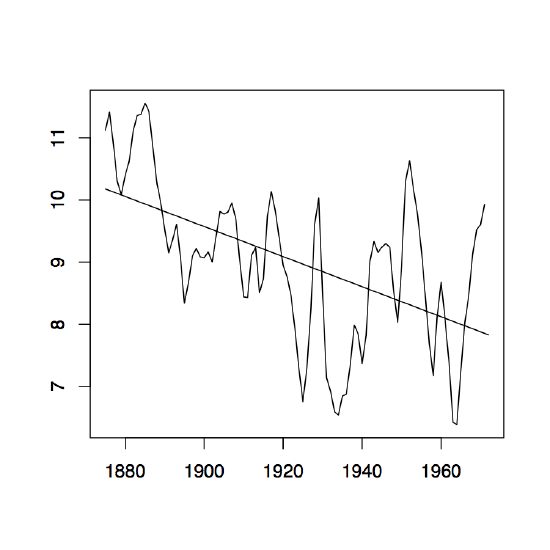
Example 1.3.1 (Level of Lake Huron). The left panel of Figure 1.7 contains the time series of the annual average water levels in feet (reduced by 570) of Lake Huron from 1875 to 1972. It is a realization of the process
\[
X_t=\mbox{(Average water level of Lake Huron in the year $1874+t$)}-570,
\qquad t=1,\ldots,98.
\nonumber \]
There seems to be a linear decline in the water level and it is therefore reasonable to fit a polynomial of order one to the data. Evaluating the least squares estimators provides us with the values

\[ \hat{b}_0=10.202 \qquad\mbox{and}\qquad \hat{b}_1=-0.0242 \nonumber \]

for the intercept and the slope, respectively. The resulting observed residuals \(\hat{y}_t=\hat{Y}_t(\omega)\) are plotted against time in the right panel of Figure 1.7. There is no apparent trend left in the data. On the other hand, the plot does not strongly support the stationarity of the residuals. Additionally, there is evidence of dependence in the data.

To reproduce the analysis in R, assume that the data is stored in the file lake.dat. Then use the following commands.

> lake = read.table("lake.dat")
> lake = ts(lake, start=1875)
> t = 1:length(lake)
> lsfit = lm(lake$^\mathrm{\sim}$t)
> plot(t, lake, xlab="", ylab="", main="")
> lines(lsfit{\$}fit)

The function lm fits a linear model or regression line to the Lake Huron data. To plot both the original data set and the fitted regression line into the same graph, you can first plot the water levels and then use the lines function to superimpose the fit. The residuals corresponding to the linear model fit can be accessed with the command lsfit$resid.

\end{exmp}

Method 2 (Smoothing with Moving Averages) Let \((X_t\colon t\in\mathbb{Z})\) be a stochastic process following model \(\ref{Eq131}\). Choose \(q\in\mathbb{N}_0\) and define the two-sided moving average
\begin{equation}\label{eq:wt}
W_t=\frac{1}{2q+1}\sum_{j=-q}^qX_{t+j}, \qquad t\in\mathbb{Z}. \tag{1.3.2}\end{equation}
The random variables \(W_t\) can be utilized to estimate the trend component \(m_t\) in the following way. First note that
\[
W_t=\frac{1}{2q+1}\sum_{j=-q}^qm_{t+j}+\frac{1}{2q+1}\sum_{j=-q}^qY_{t+j} \approx m_t,
\nonumber \]
assuming that the trend is locally approximately linear and that the average of the \(Y_t\) over the interval \([t-q,t+q]\) is close to zero. Therefore, \(m_t\) can be estimated by

\[ \hat{m}_t=W_t,\qquad t=q+1,\ldots,n-q. \nonumber \]

Notice that there is no possibility of estimating the first \(q\) and last \(n-q\) drift terms due to the two-sided nature of the moving averages. In contrast, one can also define one-sided moving averages by letting

\[ \hat{m}_1=X_1,\qquad \hat{m}_t=aX_t+(1-a)\hat{m}_{t-1},\quad t=2,\ldots,n. \nonumber \]

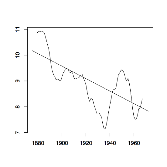
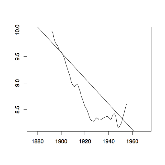
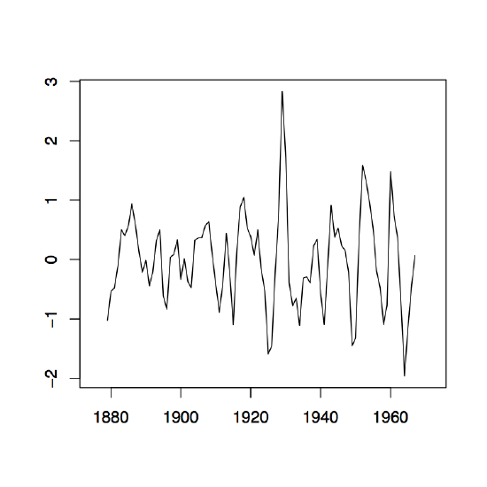
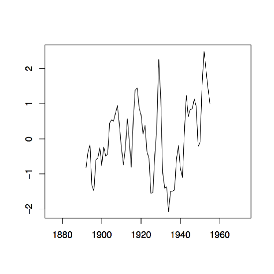
• Figure 1.8: The two-sided moving average filters Wt for the Lake Huron data (upper panel) and their residuals (lower panel) with bandwidth q = 2 (left), q = 10 (middle) and q = 35 (right).

Figure 1.8 contains estimators \(\hat{m}_t\) based on the two-sided moving averages for the Lake Huron data of Example 1.3.1. for selected choices of \(q\) (upper panel) and the corresponding estimated residuals (lower panel).

The moving average filters for this example can be produced in R in the following way:

> t = 1:length(lake)
> ma2 = filter(lake, sides=2, rep(1,5)/5)
> ma10 = filter(lake, sides=2, rep(1,21)/21)
> ma35 = filter(lake, sides=2, rep(1,71)/71)
> plot(t, ma2, xlab="", ylab="",type="l")
> lines(t,ma10); lines(t,ma35)

Therein, sides determines if a one- or two-sided filter is going to be used. The phrase rep(1,5) creates a vector of length 5 with each entry being equal to 1.

More general versions of the moving average smoothers can be obtained in the following way. Observe that in the case of the two-sided version \(W_t\) each variable \(X_{t-q},\ldots,X_{t+q}\) obtains a "weight" \(a_j=(2q+1)^{-1}\). The sum of all weights thus equals one. The same is true for the one-sided moving averages with weights \(a\) and \(1-a\). Generally, one can hence define a smoother by letting

\[\hat{m}_t=\sum_{j=-q}^qa_jX_{t+j}, \qquad t=q+1,\ldots,n-q, \tag{1.3.3} \label{Eq133} \]

where \(a_{-q}+\ldots+a_q=1\). These general moving averages (two-sided and one-sided) are commonly referred to as linear filters. There are countless choices for the weights. The one here, \(a_j=(2q+1)^{-1}\), has the advantage that linear trends pass undistorted. In the next example, a filter is introduced which passes cubic trends without distortion.

Example 1.3.2 (Spencer's 15-point moving average). Suppose that the filter in display \(\ref{Eq133}\) is defined by weights satisfying \(a_j=0\) if \(|j|>7\), \(a_j=a_{-j}\) and
\[
(a_0,a_1,\ldots,a_7)=\frac{1}{320}(74,67,46,21,3,-5,-6,-3).
\nonumber \]
Then, the corresponding filters passes cubic trends \(m_t=b_0+b_1t+b_2t^2+b_3t^3\) undistorted. To see this, observe that
\begin{align*}
\sum_{j=-7}^7a_j=1\qquad\mbox{and}\qquad
\sum_{j=-7}^7j^ra_j=0,\qquad r=1,2,3.
\end{align*}
Now apply Proposition 1.3.1 below to arrive at the conclusion. Assuming that the observations are in data, use the R commands

> a = c(-3, -6, -5, 3, 21, 46, 67, 74, 67, 46, 21, 3, -5, -6, -3)/320
> s15 = filter(data, sides=2, a)

to apply Spencer's 15-point moving average filter. This example also explains how to specify a general tailor-made filter for a given data set.

Proposition 1.3.1. A linear filter (1.3.3) passes a polynomial of degree \(p\) if and only if
\[
\sum_{j}a_j=1\qquad\mbox{and}\qquad \sum_{j}j^ra_j=0,\qquad r=1,\ldots,p.
\nonumber \]
Proof. It suffices to show that \(\sum_ja_j(t+j)^r=t^r\) for \(r=0,\ldots,p\). Using the binomial theorem, write
\begin{align*}
\sum_ja_j(t+j)^r
&=\sum_ja_j\sum_{k=0}^r{r \choose k}t^kj^{r-k}\\[.2cm]
&=\sum_{k=0}^r{r \choose k}t^k\left(\sum_ja_jj^{r-k}\right) \\[.2cm]
&=t^r
\end{align*}
for any \(r=0,\ldots,p\) if and only if the above conditions hold.

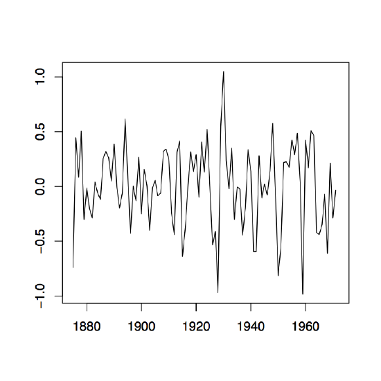
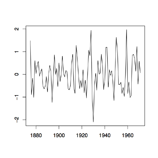
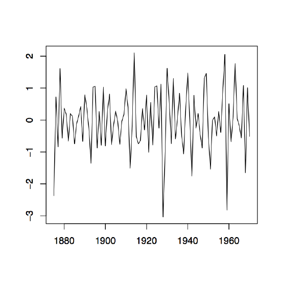
• Figure 1.9: Time series plots of the observed sequences (∇xt) in the left panel and (∇2xt) in the right panel of the differenced Lake Huron data described in Example 1.3.1.

Method 3 (Differencing) A third possibility to remove drift terms from a given time series is differencing. To this end, introduce the difference operator \(\nabla\) as
\[
\nabla X_t=X_t-X_{t-1}=(1-B)X_t, \qquad t\in T,
\nonumber \]
where \(B\) denotes the backshift operator \(BX_t=X_{t-1}\). Repeated application of \(\nabla\) is defined in the intuitive way:
\[
\nabla^2X_t=\nabla(\nabla X_t)=\nabla(X_t-X_{t-1})=X_t-2X_{t-1}+X_{t-2}
\nonumber \]
and, recursively, the representations follow also for higher powers of \(\nabla\). Suppose that the difference operator is applied to the linear trend \(m_t=b_0+b_1t\), then
\[
\nabla m_t=m_t-m_{t-1}=b_0+b_1t-b_0-b_1(t-1)=b_1
\nonumber \]
which is a constant. Inductively, this leads to the conclusion that for a polynomial drift of degree \(p\), namely \(m_t=\sum_{j=0}^pb_jt^j\), \(\nabla^pm_t=p!b_p\) and thus constant. Applying this technique to a stochastic process of the form (1.3.1) with a polynomial drift \(m_t\), yields then
\[
\nabla^pX_t=p!b_p+\nabla^p Y_t,\qquad t\in T.
\nonumber \]
This is a stationary process with mean \(p!b_p\). The plots in Figure 1.9 contain the first and second differences for the Lake Huron data. In R, they may be obtained from the commands

> d1 = diff(lake)
> d2 = diff(d1)
> par(mfrow=c(1,2))
> plot.ts(d1, xlab="", ylab="")
> plot.ts(d2, xlab="", ylab="")

The next example shows that the difference operator can also be applied to a random walk to create stationary data.

Example 1.3.3. Let \((S_t\colon t\in\mathbb{N}_0)\) be the random walk of Example 1.2.3. If the difference operator \(\nabla\) is applied to this stochastic process, then
\[
\nabla S_t=S_t-S_{t-1}=Z_t, \qquad t\in\mathbb{N}.
\nonumber \]
In other words, \(\nabla\) does nothing else but recover the original white noise sequence that was used to build the random walk.