13.9: Timid Play

Last updated
Save as PDF

Page ID: 10263

$ \newcommand{\vecs}[1]{\overset { \scriptstyle \rightharpoonup} {\mathbf{#1}} } $ $ \newcommand{\vecd}[1]{\overset{-\!-\!\rightharpoonup}{\vphantom{a}\smash {#1}}} $$\newcommand{\id}{\mathrm{id}}$ $ \newcommand{\Span}{\mathrm{span}}$ $ \newcommand{\kernel}{\mathrm{null}\,}$ $ \newcommand{\range}{\mathrm{range}\,}$ $ \newcommand{\RealPart}{\mathrm{Re}}$ $ \newcommand{\ImaginaryPart}{\mathrm{Im}}$ $ \newcommand{\Argument}{\mathrm{Arg}}$ $ \newcommand{\norm}[1]{\| #1 \|}$ $ \newcommand{\inner}[2]{\langle #1, #2 \rangle}$ $ \newcommand{\Span}{\mathrm{span}}$ $\newcommand{\id}{\mathrm{id}}$ $ \newcommand{\Span}{\mathrm{span}}$ $ \newcommand{\kernel}{\mathrm{null}\,}$ $ \newcommand{\range}{\mathrm{range}\,}$ $ \newcommand{\RealPart}{\mathrm{Re}}$ $ \newcommand{\ImaginaryPart}{\mathrm{Im}}$ $ \newcommand{\Argument}{\mathrm{Arg}}$ $ \newcommand{\norm}[1]{\| #1 \|}$ $ \newcommand{\inner}[2]{\langle #1, #2 \rangle}$ $ \newcommand{\Span}{\mathrm{span}}$$\newcommand{\AA}{\unicode[.8,0]{x212B}}$

$\newcommand{\P}{\mathbb{P}}$ $\newcommand{\E}{\mathbb{E}}$ $\newcommand{\R}{\mathbb{R}}$ $\newcommand{\N}{\mathbb{N}}$ $\newcommand{\bs}{\boldsymbol}$ $\newcommand{\var}{\text{var}}$ $\newcommand{\sd}{\text{sd}}$

Basic Theory

Recall that with the strategy of timid play in red and black, the gambler makes a small constant bet, say $1, on each game until she stops. Thus, on each game, the gambler's fortune either increases by 1 or decreases by 1, until the fortune reaches either 0 or the target $a$ (which we assume is a positive integer). Thus, the fortune process $(X_0, X_1, \ldots)$ is a random walk on the fortune space $\{0, 1, \ldots, a\}$ with 0 and $a$ as absorbing barriers.

As usual, we are interested in the probability of winning and the expected number of games. The key idea in the analysis is that after each game, the fortune process simply starts over again, but with a different initial value. This is an example of the Markov property, named for Andrei Markov. A separate chapter on Markov Chains explores these random processes in more detail. In particular, this chapter has sections on Birth-Death Chains and Random Walks on Graphs, particular classes of Markov chains that generalize the random processes that we are studying here.

Figure $\PageIndex{1}$: The transition graph for timid play

The Probability of Winning

Our analysis based on the Markov property suggests that we treat the initial fortune as a variable. Thus, we will denote the probability that the gambler reaches the target $a$, starting with an initial fortune $x$ by \[ f(x) = \P(X_N = a \mid X_0 = x), \quad x \in \{0, 1, \ldots, a\} \]

The function $f$ satisfies the following difference equation and boundary conditions:

$f(x) = q f(x - 1) + p f(x + 1)$ for $ x \in \{1, 2, \ldots, a - 1\}$
$f(0) = 0$, $f(a) = 1$

Proof

The boundary conditions are just a matter of definition. The difference equation follows from conditioning on the outcome of the first trial. She loses this trial with probability $q$ and if she loses, then effectively she starts a new sequence of trials but with initial fortune $x - 1$. She wins the first trial with probability $p$, and if she wins, then she effectively starts a new sequence of trials but with initial fortune $x + 1$.

The difference equation is linear (in the unknown function $f$), homogeneous (because each term involves the unknown function $f$), and second order (because 2 is the difference between the largest and smallest fortunes in the equation). Recall that linear homogeneous difference equations can be solved by finding the roots of the characteristic equation.

The characteristic equation of the difference equation is $p r^2 - r + q = 0$, and that the roots are $r = 1$ and $r = q / p$.

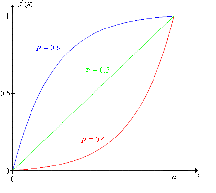
If $p \ne \frac{1}{2}$, then the roots are distinct. In this case, the probability that the gambler reaches her target is \[ f(x) = \frac{(q / p)^x - 1}{(q / p)^a - 1}, \quad x \in \{0, 1, \ldots, a\} \]

If $p = \frac{1}{2}$, the characteristic equation has a single root 1 that has multiplicity 2. In this case, the probability that the gambler reaches her target is simply the ratio of the initial fortune to the target fortune: \[ f(x) = \frac{x}{a}, \quad x \in \{0, 1, \ldots, a\} \]

Thus, we have the distribution of the final fortune $X_N$ in either casse: \[ \P(X_N = 0 \mid X_0 = x) = 1 - f(x), \; \P(X_N = a \mid X_0 = x) = f(x); \quad x \in \{0, 1, \ldots, a\} \]

In the red and black experiment, choose Timid Play. Vary the initial fortune, target fortune, and game win probability and note how the probability of winning the game changes. For various values of the parameters, run the experiment 1000 times and compare the relative frequency of winning a game to the probability of winning a game.

As a function of $x$, for fixed $p$ and $a$,

$f$ is increasing from 0 to $a$.
$f$ is concave upward if $p \lt \frac{1}{2}$ and concave downward if $p \gt \frac{1}{2}$. Of course, $f$ is linear if $p = \frac{1}{2}$.

$f$ is continuous as a function of $p$, for fixed $x$ and $a$.

Proof

An application of L'Hospital's Rule shows that the probability of winning when $ p \ne \frac{1}{2} $ converges to the probability of winning when $ p = \frac{1}{2} $, as $p \to \frac{1}{2}$.

For fixed $x$ and $a$, $f(x)$ increases from 0 to 1 as $p$ increases from 0 to 1.

Figure $\PageIndex{2}$: The graph of $f$ for $p = 0.4$, $p = 0.5$, and $p = 0.6$

The Expected Number of Trials

Now let us consider the expected number of games needed with timid play, when the initial fortune is $x$: \[ g(x) = \E(N \mid X_0 = x), \quad x \in \{0, 1, \ldots, a\} \]

The function $g$ satisfies the following difference equation and boundary conditions:

$g(x) = q g(x - 1) + p g(x + 1) + 1$ for $ x \in \{1, 2, \ldots, a - 1\}$
$g(0) = 0$, $g(a) = 0$

Proof

Again, the difference equation follows from conditioning on the first trial. She loses this trial with probability $q$ and if she loses, then effectively she starts a new sequence of trials but with initial fortune $x - 1$. She wins the first trial with probability $p$, and if she wins, then she effectively starts a new sequence of trials but with initial fortune $x + 1$. In either case, one trial is over.

The difference equation in the last exercise is linear, second order, but non-homogeneous (because of the constant term 1 on the right side). The corresponding homogeneous equation is the equation satisfied by the win probability function $f$. Thus, only a little additional work is needed to solve the non-homogeneous equation.

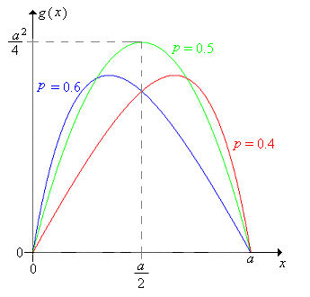
If $p \ne \frac{1}{2}$, then \[ g(x) = \frac{x}{q - p} - \frac{a}{q - p} f(x), \quad x \in \{0, 1, \ldots, a\} \] where $f$ is the win probability function above.

If $p = \frac{1}{2}$, then \[ g(x) = x (a - x), \quad x \in \{0, 1, \ldots, a\} \]

Consider $g$ as a function of the initial fortune $x$, for fixed values of the game win probability $p$ and the target fortune $a$.

$g$ at first increases and then decreases.
$g$ is concave downward.

When $ p = \frac{1}{2} $, the maximum value of $ g $ is $ \frac{a^2}{4} $ and occurs when $ x = \frac{a}{2} $. When $p \ne \frac{1}{2}$, the value of $x$ where the maximum occurs is rather complicated.

Figure $\PageIndex{3}$: The graph of $g$ for $p = 0.4$, $p = 0.5$, and $p = 0.6$

$g$ is continuous as a function of $p$, for fixed $x$ and $a$.

Proof

The expected value when $ p \ne \frac{1}{2} $ converges to the expected value when $ p = \frac{1}{2} $, as $p \to \frac{1}{2}$.

For many parameter settings, the expected number of games is surprisingly large. For example, suppose that $p = \frac{1}{2}$ and the target fortune is 100. If the gambler's initial fortune is 1, then the expected number of games is 99, even though half of the time, the gambler will be ruined on the first game. If the initial fortune is 50, the expected number of games is 2500.

In the red and black experiment, select Timid Play. Vary the initial fortune, the target fortune and the game win probability and notice how the expected number of games changes. For various values of the parameters, run the experiment 1000 times and compare the sample mean number of games to the expect value.

Increasing the Bet

What happens if the gambler makes constant bets, but with an amount higher than 1? The answer to this question may give insight into what will happen with bold play.

In the red and black game, set the target fortune to 16, the initial fortune to 8, and the win probability to 0.45. Play 10 games with each of the following strategies. Which seems to work best?

Bet 1 on each game (timid play).
Bet 2 on each game.
Bet 4 on each game.
Bet 8 on each game (bold play).

We will need to embellish our notation to indicate the dependence on the target fortune. Let \[ f(x, a) = \P(X_N = a \mid X_0 = x), \quad x \in \{0, 1, \ldots, a\}, \; a \in \N_+ \] Now fix $p$ and suppose that the target fortune is $2 a$ and the initial fortune is $2 x$. If the gambler plays timidly (betting $1 each time), then of course, her probability of reaching the target is $f(2 x, 2 a)$. On the other hand:

Suppose that the gambler bets $2 on each game. The fortune process $(X_i / 2: i \in \N)$ corresponds to timid play with initial fortune $x$ and target fortune $a$ and that therefore the probability that the gambler reaches the target is $f(x, a)$.

Thus, we need to compare the probabilities $f(2 x, 2 a)$ and $f(x, a)$.

The win probability functions are related as follows: \[ f(2 x, 2 a) = f(x, a) \frac{(q / p)^x + 1}{(q / p)^a + 1}, \quad x \in \{0, 1, \ldots, a\} \] In particular

$f(2 x, 2 a) \lt f(x, a)$ if $p \lt \frac{1}{2}$
$f(2 x, 2 a) = f(x, a)$ if $p = \frac{1}{2}$
$f(2 x, 2 a) \gt f(x, a)$ if $p \gt \frac{1}{2}$

Thus, it appears that increasing the bets is a good idea if the games are unfair, a bad idea if the games are favorable, and makes no difference if the games are fair.

What about the expected number of games played? It seems almost obvious that if the bets are increased, the expected number of games played should decrease, but a direct analysis using the expected value function above is harder than one might hope (try it!), We will use a different method, one that actually gives better results. Specifically, we will have the $1 and $2 gamblers bet on the same underlying sequence of games, so that the two fortune processes are defined on the same sample space. Then we can compare the actual random variables (the number of games played), which in turn leads to a comparison of their expected values. Recall that this general method is referred to as coupling.

Let $X_n$ denote the fortune after $n$ games for the gamble making $1 bets (simple timid play). Then $2 X_n - X_0$ is the fortune after $n$ games for the gambler making $2 bets (with the same initial fortune, betting on the same sequence of games). Assume again that the initial fortune is $2 x$ and the target fortune $2 a$ where $0 \lt x \lt a$. Let $N_1$ denote the number of games played by the $1 gambler, and $N_2$ the number of games played by the $2 gambler, Then

If the $1 gambler falls to fortune $x$, the $2 gambler is ruined (fortune 0).
If the $1 gambler hits fortune $x + a$, the $2 gambler reaches the target $2 a$.
The $1 gambler must hit $x$ before hitting 0 and must hit $x + a$ before hitting $2 a$.
$N_2 \lt N_1$ given $X_0 = 2 x$.
$\E(N_2 \mid X_0 = 2 x) \lt \E(N_1 \mid X_0 = 2 x)$

Of course, the expected values agree (and are both 0) if $x = 0$ or $x = a$. This result shows that $N_2$ is stochastically smaller than $N_1$ when the gamblers are not playing the same sequence of games (so that the random variables are not defined on the same sample space).

Generalize the analysis in this subsection to compare timid play with the strategy of betting $$k$ on each game (let the initial fortune be $k x$ and the target fortune $k a$.

It appears that with unfair games, the larger the bets the better, at least in terms of the probability of reaching the target. Thus, we are naturally led to consider bold play.