12.4: Order Statistics

\(\newcommand{\P}{\mathbb{P}}\) \(\newcommand{\E}{\mathbb{E}}\) \(\newcommand{\R}{\mathbb{R}}\) \(\newcommand{\N}{\mathbb{N}}\) \(\newcommand{\bs}{\boldsymbol}\) \(\newcommand{\var}{\text{var}}\) \(\newcommand{\cov}{\text{cov}}\) \(\newcommand{\cor}{\text{cor}}\)

Basic Theory

Definitions

Suppose that the objects in our population are numbered from 1 to \(m\), so that \(D = \{1, 2, \ldots, m\}\). For example, the population might consist of manufactured items, and the labels might correspond to serial numbers. As in the basic sampling model we select \(n\) objects at random, without replacement from \(D\). Thus the outcome is \(\bs{X} = (X_1, X_2, \ldots, X_n)\) where \(X_i \in S\) is the \(i\)th object chosen. Recall that \(\bs{X}\) is uniformly distributed over the set of permutations of size \(n\) chosen from \(D\). Recall also that \(\bs{W} = \{X_1, X_2, \ldots, X_n\}\) is the unordered sample, which is uniformly distributed on the set of combinations of size \(n\) chosen from \(D\).

For \(i \in \{1, 2, \ldots, n\}\) let \(X_{(i)} = i\)th smallest element of \(\{X_1, X_2, \ldots, X_n\}\). The random variable \(X_{(i)}\) is known as the order statistic of order \(i\) for the sample \(\bs{X}\). In particular, the extreme order statistics are \begin{align} X_{(1)} & = \min\{X_1, X_2, \ldots, X_n\} \\ X_{(n)} & = \max\{X_1, X_2, \ldots, X_n\} \end{align} Random variable \(X_{(i)}\) takes values in \(\{i, i + 1, \ldots, m - n + i\}\) for \( i \in \{1, 2, \ldots, n\} \).

We will denote the vector of order statistics by \(\bs{Y} = \left(X_{(1)}, X_{(2)}, \ldots, X_{(n)}\right)\). Note that \(\bs{Y}\) takes values in \[ L = \left\{(y_1, y_2, \ldots, y_n) \in D^n: y_1 \lt y_2 \lt \cdots \lt y_n\right\} \]

Run the order statistic experiment. Note that you can vary the population size \(m\) and the sample size \(n\). The order statistics are recorded on each update.

Distributions

\(L\) has \(\binom{m}{n}\) elements and \(\bs{Y}\) is uniformly distributed on \(L\).

Proof

For \(\bs{y} = (y_1, y_2, \ldots, y_n) \in L\), \(\bs{Y} = \bs{y}\) if and only if \(\bs{X}\) is one of the \(n!\) permutations of \(\bs{y}\). Hence \(\P(\bs{Y} = \bs{y}) = n! \big/ m^{(n)} = 1 \big/ \binom{m}{n}\).

The probability density function of \(X_{(i)}\) is \[ \P\left[X_{(i)} = x\right] = \frac{\binom{x-1}{i-1} \binom{m-x}{n-i}}{\binom{m}{n}}, \quad x \in \{i, i + 1, \ldots, m - n + i\} \]

Proof

The event that the \(i\)th order statistic is \(x\) means that \(i - 1\) sample values are less than \(x\) and \(n - i\) are greater than \(x\), and of course, one of the sample values is \(x\). By the multiplication principle of combinatorics, the number of unordered samples corresponding to this event is \(\binom{x-1}{i-1} \binom{m - x}{n - i}\). The total number of unordered samples is \(\binom{m}{n}\).

In the order statistic experiment, vary the parameters and note the shape and location of the probability density function. For selected values of the parameters, run the experiment 1000 times and compare the relative frequency function to the probability density function.

Moments

The probability density function of \( X_{(i)} \) above can be used to obtain an interesting identity involving the binomial coefficients. This identity, in turn, can be used to find the mean and variance of \(X_{(i)}\).

For \(i, \, n, \, m \in \N_+\) with \(i \le n \le m\), \[ \sum_{k=i}^{m-n+i} \binom{k-1}{i-1} \binom{m-k}{n - i} = \binom{m}{n} \]

Proof

This result follows immediately from the probability density function of \( X_{(i)} \) above

The expected value of \(X_{(i)}\) is \[ \E\left[X_{(i)}\right] = i \frac{m + 1}{n+1}\]

Proof

We start with the definition of expected value. Recall that \(x \binom{x - 1}{i - 1} = i \binom{x}{i}\). Next we use the identity above with \(m\) replaced with \(m + 1\), \(n\) replaced with \(n + 1\), and \(i\) replaced with \(i + 1\). Simplifying gives the result.

The variance of \(X_{(i)}\) is \[ \var\left[X_{(i)}\right] = i (n - i + 1) \frac{(m + 1) (m - n)}{(n + 1)^2 (n + 2)} \]

Proof

The result follows from another application of the identity above.

In the order statistic experiment, vary the parameters and note the size and location of the mean \( \pm \) standard deviation bar. For selected values of the parameters, run the experiment 1000 times and compare the sample mean and standard deviation to the distribution mean and standard deviation.

Estimators of \( m \) Based on Order Statistics

Suppose that the population size \( m \) is unknown. In this subsection we consider estimators of \( m \) constructed from the various order statistics.

For \(i \in \{1, 2, \ldots, n\}\), the following statistic is an unbiased estimator of \(m\): \[ U_i = \frac{n + 1}{i} X_{(i)} - 1 \]

Proof

From the expected value of \( X_{(i)} \) above and the linear property of expected value, note that \(\E(U_i) = m\).

Since \(U_i\) is unbiased, its variance is the mean square error, a measure of the quality of the estimator.

The variance of \(U_i\) is \[ \var(U_i) = \frac{(m + 1) (m - n) (n - i +1)}{i (n + 2)}\]

Proof

This result follows from variance of \( X_{(i)} \) given above and standard properties of variance.

For fixed \(m\) and \(n\), \(\var(U_i)\) decreases as \(i\) increases. Thus, the estimators improve as \(i\) increases; in particular, \(U_n\) is the best and \(U_1\) the worst.

The relative efficiency of \(U_j\) with respect to \(U_i\) is \[ \frac{\var(U_i)}{\var(U_j)} = \frac{j (n - i + 1)}{i (n - j + 1)} \]

Note that the relative efficiency depends only on the orders \(i\) and \(j\) and the sample size \(n\), but not on the population size \(m\) (the unknown parameter). In particular, the relative efficiency of \(U_n\) with respect to \(U_1\) is \(n^2\). For fixed \( i \) and \( j \), the asymptotic relative efficiency of \( U_j \) to \( U_i \) is \( j / i \). Usually, we hope that an estimator improves (in the sense of mean square error) as the sample size \(n\) increases (the more information we have, the better our estimate should be). This general idea is known as consistency.

\(\var(U_n)\) decreases to 0 as \(n\) increases from 1 to \(m\), and so \(U_n\) is consistent: \[ \var(U_n) = \frac{(m + 1)(m - n)}{n (n + 2)} \]

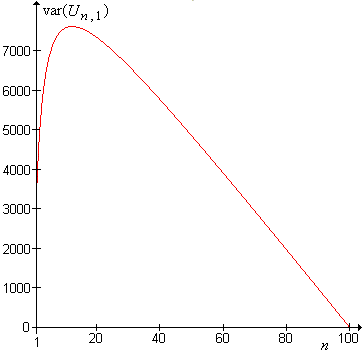
For fixed \(i\), \(\var(U_i)\) at first increases and then decreases to 0 as \(n\) increases from \(i\) to \(m\). Thus, \(U_i\) is inconsistent.

Figure \(\PageIndex{1}\): \(\var(U_1)\) as a function of \(n\) for \(m = 100\)

An Estimator of \(m\) Based on the Sample Mean

In this subsection, we will derive another estimator of the parameter \(m\) based on the average of the sample variables \(M = \frac{1}{n} \sum_{i=1}^n x_i\), (the sample mean) and compare this estimator with the estimator based on the maximum of the variables (the largest order statistic).

\(\E(M) = \frac{m + 1}{2}\).

Proof

Recall that \(X_i\) is uniformly distributed on \(D\) for each \(i\) and hence \(\E(X_i) = \frac{m + 1}{2}\).

It follows that \(V = 2 M - 1\) is an unbiased estimator of \(m\). Moreover, it seems that superficially at least, \(V\) uses more information from the sample (since it involves all of the sample variables) than \(U_n\). Could it be better? To find out, we need to compute the variance of the estimator (which, since it is unbiased, is the mean square error). This computation is a bit complicated since the sample variables are dependent. We will compute the variance of the sum as the sum of all of the pairwise covariances.

For distinct \(i, \, j \in \{1, 2, \ldots, n\}\), \(\cov\left(X_i, X_j\right) = -\frac{m+1}{12}\).

Proof

First recall that given \(X_i = x\), \(X_j\) is uniformly distributed on \(D \setminus \{x\}\). Hence \(\E(X_j \mid X_i = x) = \frac{m(m + 1)}{2 (m - 1)} - \frac{x}{m - 1}\). Thus conditioning on \(X_i\) gives \(\E(X_i X_j) = \frac{(m +1)(3 \, m + 2)}{12}\). The result now follows from the standard formula \(\cov(X_i, X_j) = \E(X_i X_j) - \E(X_i) \E(X_j)\).

For \(i \in \{1, 2, \ldots, n\}\), \(\var(X_i) = \frac{m^2 - 1}{12}\).

Proof

This follows since \(X_i\) is uniformly distributed on \(D\).

\(\var(M) = \frac{(m+1)(m-n)}{12 \, n}\).

Proof

The variance of \(M\) is \(\frac{1}{n^2}\) times the sum of \(\cov\left(X_i, X_j\right)\) over all \(i, \, j \in \{1, 2, \ldots, n\}\). There are \(n\) covariance terms with the value given in the variance result above (corresponding to \( i = j \)) and \(n^2 - n\) terms with the value given in the pure covariance result above (corresponding to \( i \ne j \)). Simplifying gives the result.

\(\var(V) = \frac{(m + 1)(m - n)}{3 \, n}\).

Proof

This follows from the variance of \( M \) above and standard properties of variance.

The variance of \( V \) is decreasing with \(n\), so \(V\) is also consistent. Let's compute the relative efficiency of the estimator based on the maximum to the estimator based on the mean.

\(\var(V) \big/ \var(U_n) = (n + 2) / 3\).

Thus, once again, the estimator based on the maximum is better. In addition to the mathematical analysis, all of the estimators except \(U_n\) can sometimes be manifestly worthless by giving estimates that are smaller than some of the smaple values.

Sampling with Replacement

If the sampling is with replacement, then the sample \(\bs{X} = (X_1, X_2, \ldots, X_n)\) is a sequence of independent and identically distributed random variables. The order statistics from such samples are studied in the chapter on Random Samples.

Examples and Applications

Suppose that in a lottery, tickets numbered from 1 to 25 are placed in a bowl. Five tickets are chosen at random and without replacement.

1. Find the probability density function of \(X_{(3)}\).
2. Find \(\E\left[X_{(3)}\right]\).
3. Find \(\var\left[X_{(3)}\right]\).

Answer

1. \(\P\left[X_{(3)} = x\right] = \frac{\binom{x-1}{2} \binom{25-x}{2}}{\binom{25}{5}}\) for \(x \in \{3, 4, \ldots, 23\}\)
2. \(\E\left[X_{(3)}\right] = 13\)
3. \(\var\left[X_{(3)}\right] = \frac{130}{7}\)

The German Tank Problem

The estimator \(U_n\) was used by the Allies during World War II to estimate the number of German tanks \(m\) that had been produced. German tanks had serial numbers, and captured German tanks and records formed the sample data. The statistical estimates turned out to be much more accurate than intelligence estimates. Some of the data are given in the table below.

German Tank Data. Source: Wikipedia

Date	Statistical Estimate	Intelligence Estimate	German Records
June 1940	169	1000	122
June 1941	244	1550	271
August 1942	327	1550	342

One of the morals, evidently, is not to put serial numbers on your weapons!

Suppose that in a certain war, 5 enemy tanks have been captured. The serial numbers are 51, 3, 27, 82, 65. Compute the estimate of \(m\), the total number of tanks, using all of the estimators discussed above.

Answer

1. \(u_1 = 17\)
2. \(u_2 = 80\)
3. \(u_3 = 101\)
4. \(u_4 = 96.5\)
5. \(u_5 = 97.4\)
6. \(v = 90.2\)

In the order statistic experiment, and set \(m = 100\) and \(n = 10\). Run the experiment 50 times. For each run, compute the estimate of \(m\) based on each order statistic. For each estimator, compute the square root of the average of the squares of the errors over the 50 runs. Based on these empirical error estimates, rank the estimators of \(m\) in terms of quality.

Suppose that in a certain war, 10 enemy tanks have been captured. The serial numbers are 304, 125, 417, 226, 192, 340, 468, 499, 87, 352. Compute the estimate of \(m\), the total number of tanks, using the estimator based on the maximum and the estimator based on the mean.

Answer

1. \(u = 548\)
2. \(v = 601\)