10.2: Bertrand's Paradox

\(\newcommand{\P}{\mathbb{P}}\) \(\newcommand{\E}{\mathbb{E}}\) \(\newcommand{\var}{\text{var}}\) \(\newcommand{\R}{\mathbb{R}}\) \(\newcommand{\N}{\mathbb{N}}\) \(\newcommand{\area}{\text{area}}\)

Preliminaries

Statement of the Problem

Bertrand's problem is to find the probability that a random chord on a circle will be longer than the length of a side of the inscribed equilateral triangle. The problem is named after the French mathematician Joseph Louis Bertrand, who studied the problem in 1889.

It turns out, as we will see, that there are (at least) three answers to Bertrand's problem, depending on how one interprets the phrase random chord. The lack of a unique answer was considered a paradox at the time, because it was assumed (naively, in hindsight) that there should be a single natural answer.

Run Bertrand's experiment 100 times for each of the following models. Do not be concerned with the exact meaning of the models, but see if you can detect a difference in the behavior of the outcomes

1. Uniform distance
2. Uniform angle
3. Uniform endpoint

Mathematical Formulation

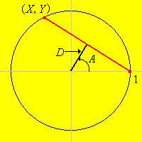
To formulate the problem mathematically, let us take \((0, 0)\) as the center of the circle and take the radius of the circle to be 1. These assumptions entail no loss of generality because they amount to measuring distances relative to the center of the circle, and taking the radius of the circle as the unit of length. Now consider a chord on the circle. By rotating the circle, we can assume that one point of the chord is \((1, 0)\) and the other point is \((X, Y)\) where \(Y \gt 0\) and \(X^2 + Y^2 = 1\).

With these assumptions, the chord is completely specified by giving any one of the following variables

1. The (perpendicular) distance \(D\) from the center of the circle to the midpoint of the chord. Note that \(0 \le D \le 1\).
2. The angle \(A\) between the \(x\)-axis and the line from the center of the circle to the midpoint of the chord. Note that \(0 \le A \le \pi / 2\).
3. The horizontal coordinate \(X\). Note that \(-1 \le X \le 1\).

Figure \(\PageIndex{1}\): A chord in the circle

The variables are related as follows:

1. \(D = \cos(A)\)
2. \(X = 2 D^2 - 1\)
3. \(Y = 2 D \sqrt{1 - D^2}\)

The inverse relations are given below. Note again that there are one-to-one correspondences between \(X\), \(A\), and \(D\).

1. \(A = \arccos(D)\)
2. \(D = \sqrt{\frac{1}{2}(x + 1)}\)
3. \(D = \sqrt{\frac{1}{2} \pm \frac{1}{2} \sqrt{1 - y^2} }\)

If the chord is generated in a probabilistic way, \(D\), \(A\), \(X\), and \(Y\) become random variables. In light of the previous results, specifying the distribution of any of the variables \(D\), \(A\), or \(X\) completely determines the distribution of all four variables.

The angle \(A\) is also the angle between the chord and the tangent line to the circle at \((1, 0)\).

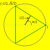
Now consider the equilateral triangle inscribed in the circle so that one of the vertices is \((1, 0)\). Consider the chord defined by the upper side of the triangle.

For this chord, the angle, distance, and coordinate variables are given as follows:

1. \(a = \pi / 3\)
2. \(d = 1 / 2\)
3. \(x = -1 / 2\)
4. \(y = \sqrt{3} / 2\)

Figure \(\PageIndex{2}\): The inscribed equilateral triangle

Now suppose that a chord is chosen in probabilistic way.

The length of the chord is greater than the length of a side of the inscribed equilateral triangle if and only if the following equivalent conditions occur:

1. \(0 \lt D \lt 1 / 2\)
2. \(\pi / 3 \lt A \lt \pi / 2\)
3. \(-1 \lt X \lt -1 / 2\)

Models

When an object is generated at random, a sequence of natural variables that determines the object should be given an appropriate uniform distribution. The coordinates of the coin center are such a sequence in Buffon's coin experiment; the angle and distance variables are such a sequence in Buffon's needle experiment. The crux of Bertrand's paradox is the fact that the distance \(D\), the angle \(A\), and the coordinate \(X\) each seems to be a natural variable that determine the chord, but different models are obtained, depending on which is given the uniform distribution.

The Model with Uniform Distance

Suppose that \(D\) is uniformly distributed on the interval \([0, 1]\).

The solution of Bertrand's problem is \[ \P \left( D \lt \frac{1}{2} \right) = \frac{1}{2} \]

In Bertrand's experiment, select the uniform distance model. Run the experiment 1000 times and compare the relative frequency function of the chord event to the true probability.

The angle \(A\) has probability density function \[ g(a) = \sin(a), \quad 0 \lt a \lt \frac{\pi}{2} \]

Proof

This follows from the standard the change of variables formula.

The coordinate \(X\) has probability density function \[ h(x) = \frac{1}{\sqrt{8 (x + 1)}}, \quad -1 \lt x \lt 1 \]

Proof

This follows from the standard the change of variables formula.

Note that \(A\) and \(X\) do not have uniform distributions. Recall that a random number is a simulation of a variable with the standard uniform distribution, that is the continuous uniform distribution on the interval \( [0, 1) \).

Show how to simulate \(D\), \(A\), \(X\), and \(Y\) using a random number.

Answer

\(A = \arccos(D)\), \(X = 2 D^2 - 1\), \(Y = 2 D \sqrt{1 - D^2}\), where \(D\) is a random number

The Model with Uniform Angle

Suppose that \(A\) is uniformly distributed on the interval \((0, \pi / 2)\).

The solution of Bertrand's problem is \[ \P\left(A \gt \frac{\pi}{3} \right) = \frac{1}{3} \]

In Bertrand's experiment, select the uniform angle model. Run the experiment 1000 times and compare the relative frequency function of the chord event to the true probability.

The distance \(D\) has probability density function \[ f(d) = \frac{2}{\pi \sqrt{1 - d^2}}, \quad 0 \lt d \lt 1 \]

Proof

This follows from the standard change of variables formula.

The coordinate \(X\) has probability density function \[ h(x) = \frac{1}{\pi \sqrt{1 - x^2}}, \quad -1 \lt x \lt 1 \]

Proof

This follows from the change of variables formula.

Note that \(D\) and \(X\) do not have uniform distributions.

Show how to simulate \(D\), \(A\), \(X\), and \(Y\) using a random number.

Answer

\(A = \frac{\pi}{2} U\), \(D = \cos(A)\), \(X = 2 D^2 - 1\), \(Y = 2 D \sqrt{1 - D^2}\), where \(U\) is a random number.

The Model with Uniform Endpoint

Suppose that \(X\) is uniformly distributed on the interval \((-1, 1)\).

The solution of Bertrand's problem is \[ \P \left( -1 \lt X \lt -\frac{1}{2} \right) = \frac{1}{4} \]

In Bertrand's experiment, select the uniform endpoint model. Run the experiment 1000 times and compare the relative frequency function of the chord event to the true probability.

The distance \(D\) has probability density function \[ f(d) = 2 d, \quad 0 \lt d \lt 1 \]

Proof

This follows from the change of variables formula.

The angle \(A\) has probability density function \[ g(a) = 2 \sin(a) \cos(a), \quad 0 \lt a \lt \frac{\pi}{2} \]

Proof

This follows from the change of variables formula.

Note that \(D\) and \(A\) do not have uniform distributions; in fact, \(D\) has a beta distribution with left parameter 2 and right parameter 1.

Physical Experiments

Suppose that a random chord is generated by tossing a coin of radius 1 on a table ruled with parallel lines that are distance 2 apart. Which of the models (if any) would apply to this physical experiment?

Answer

Uniform distance

Suppose that a needle is attached to the edge of disk of radius 1. A random chord is generated by spinning the needle. Which of the models (if any) would apply to this physical experiment?

Answer

Uniform angle

Suppose that a thin trough is constructed on the edge of a disk of radius 1. Rolling a ball in the trough generates a random point on the circle, so a random chord is generated by rolling the ball twice. Which of the models (if any) would apply to this physical experiment?

Answer

Uniform angle